Store your data with KnowPulse
Overview
Teaching: 10 min
Exercises: 20 minQuestions
How do I store my raw phenotypic data in KnowPulse?
Objectives
Backup your raw phenotypic data to KnowPulse.
Welcome to KnowPulse
KnowPulse can be used to store your raw phenotypic data; we highly recommend backing up your data regularly in KnowPulse during the growing season.
Upload your data files
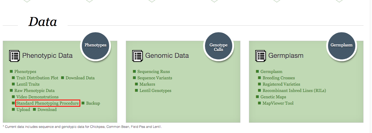
Scroll down to the Data section, in the Phenotypic Data box, there are Video Demonstrations to guide you for data upload. In these demonstration videos, you will learn the phenotypic data functionality that is available on KnowPulse.
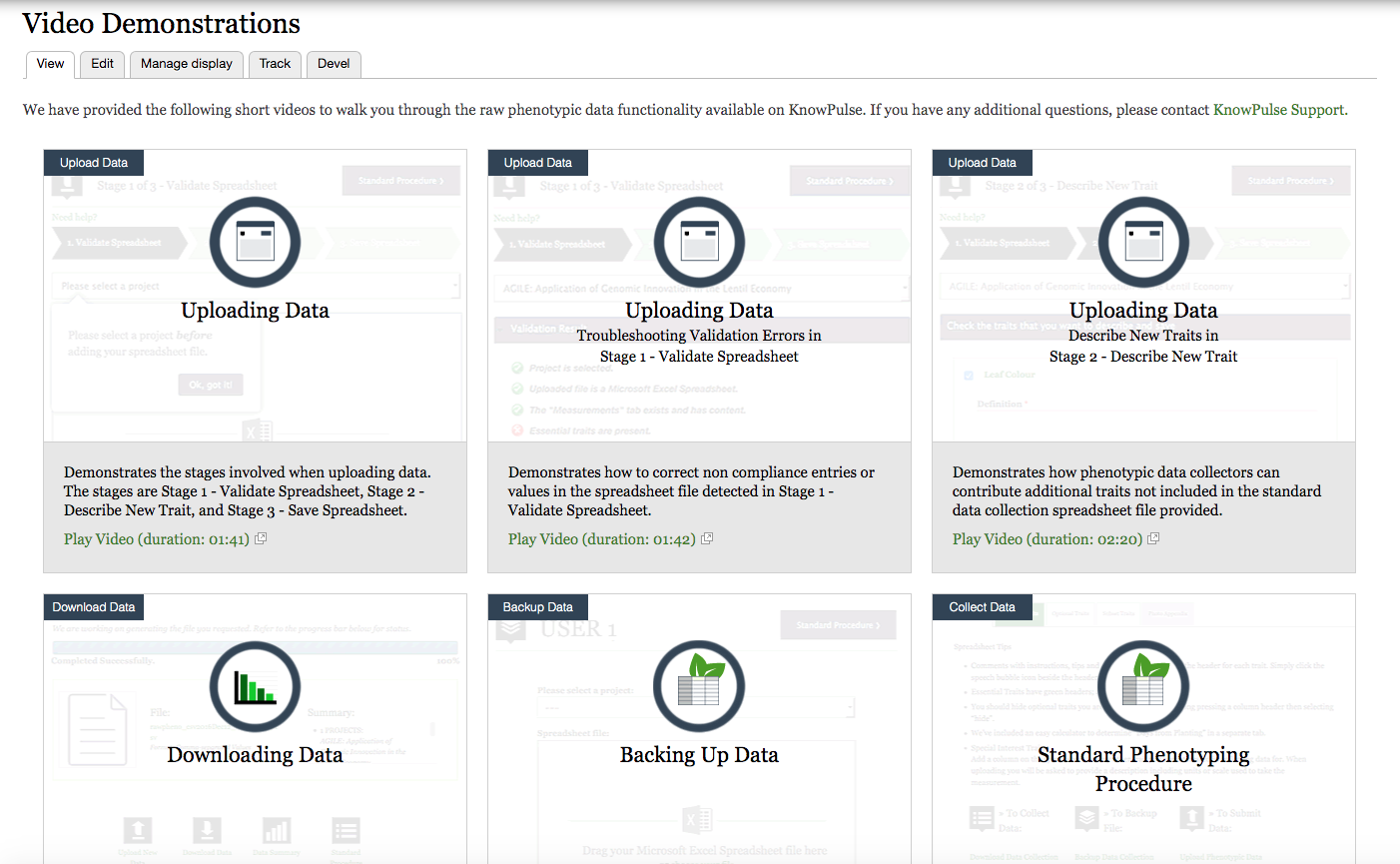
If you are already familiar with the standard phenotyping procedures, you can have your raw phenotypic data backup, upload, and download from here.
Your data is kept confidential with us until you are ready to publish them.
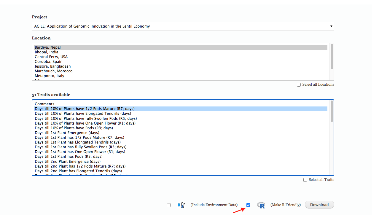
At the end of the season, you can download your data with an R-friendly header from KnowPulse.
Key Points
Make sure you download and use the standard data collection template for your data.
Remember to backup your data with KnowPulse regularly during the growing season.
Download your data files with an R-friendly header.
Import data into R
Overview
Teaching: 20 min
Exercises: 20 minQuestions
How to get my data file into R?
Objectives
Import your .csv file to RStudio with its Url.
Import your .csv file to RStudio with command.
Two options to let RStudio read your data
After the growing season, you have your data downloaded from KnowPulse in a comma separated value .csv format file. In the next step, you want to import your .csv file into Rstudio for further analysis.
RStudio can read files in various formats, see Importing Data with RStudio for more details.
Option 1: Import your .csv file with its path
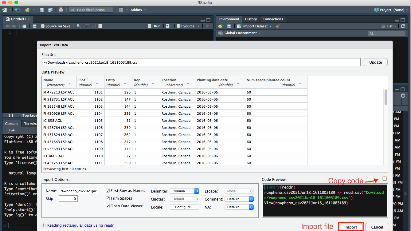
Step 1
Import your downloaded .csv file on bottom right panel to Rstudio, so you will be able to see the Url of your file.
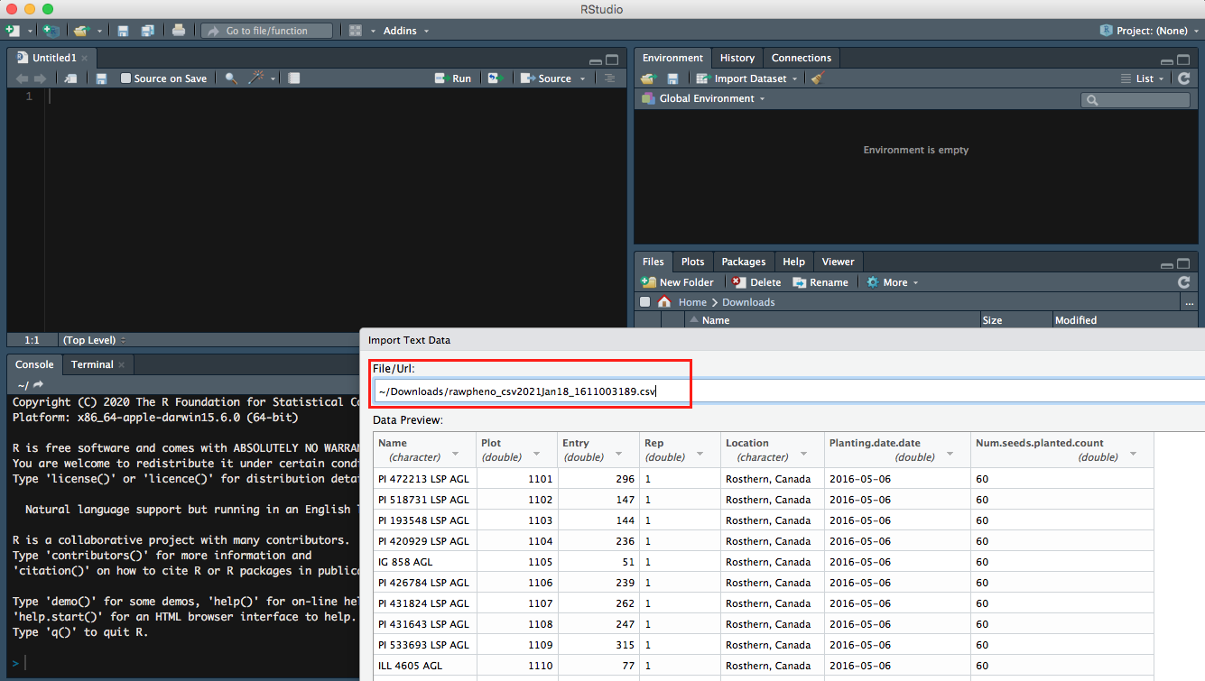
Step 2
Then you can preview your data; meanwhile, more Import Options are available for you to rename your file or choose which sheet you would like RStudio to view if your file has multiple pages.
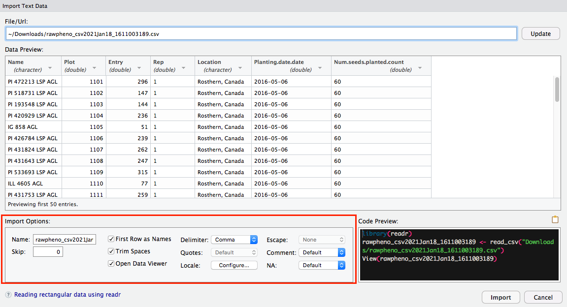
Step 3
It is intuitive to hit Import button, which is an option to import your file; as an alternate, you can also copy-paste the code into the editor panel.
Step 4
Inside the bracket beside the library, readr is the package that is used to read your file. So you want to run both lines of code.
- Two ways to run your code in a script:
- Select the line, then click the run button on top right in editor panel
- shortcut
- Mac users:
command+enter - Windows users:
control+enter
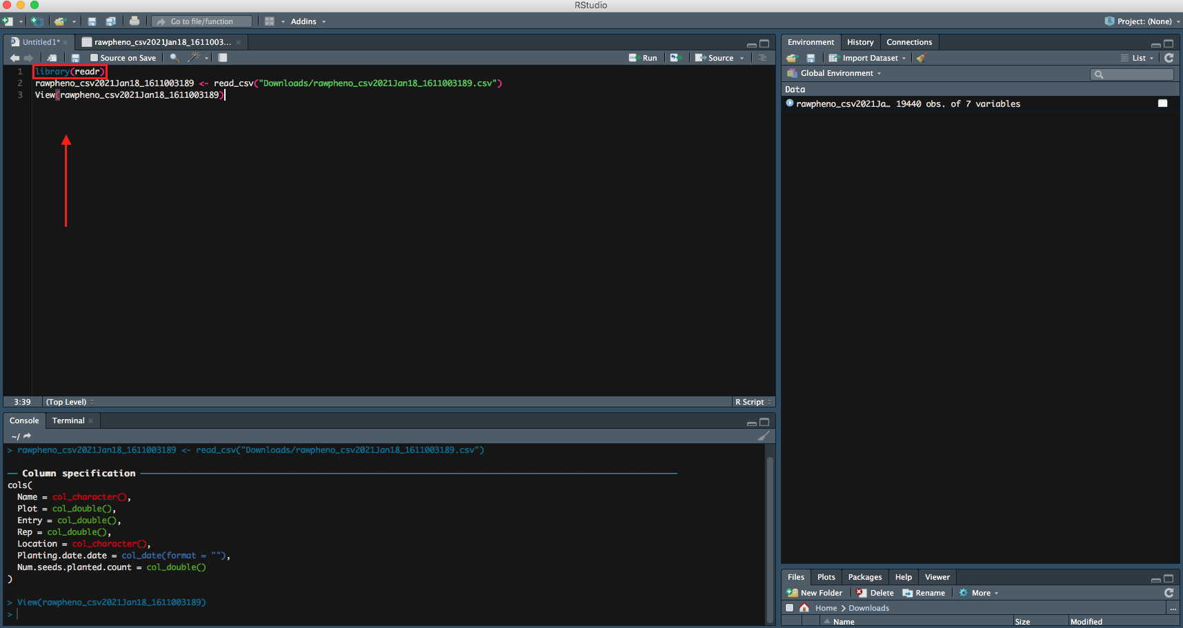
Right now, your file is successfully imported to RStudio; you can continue on your data analysis.
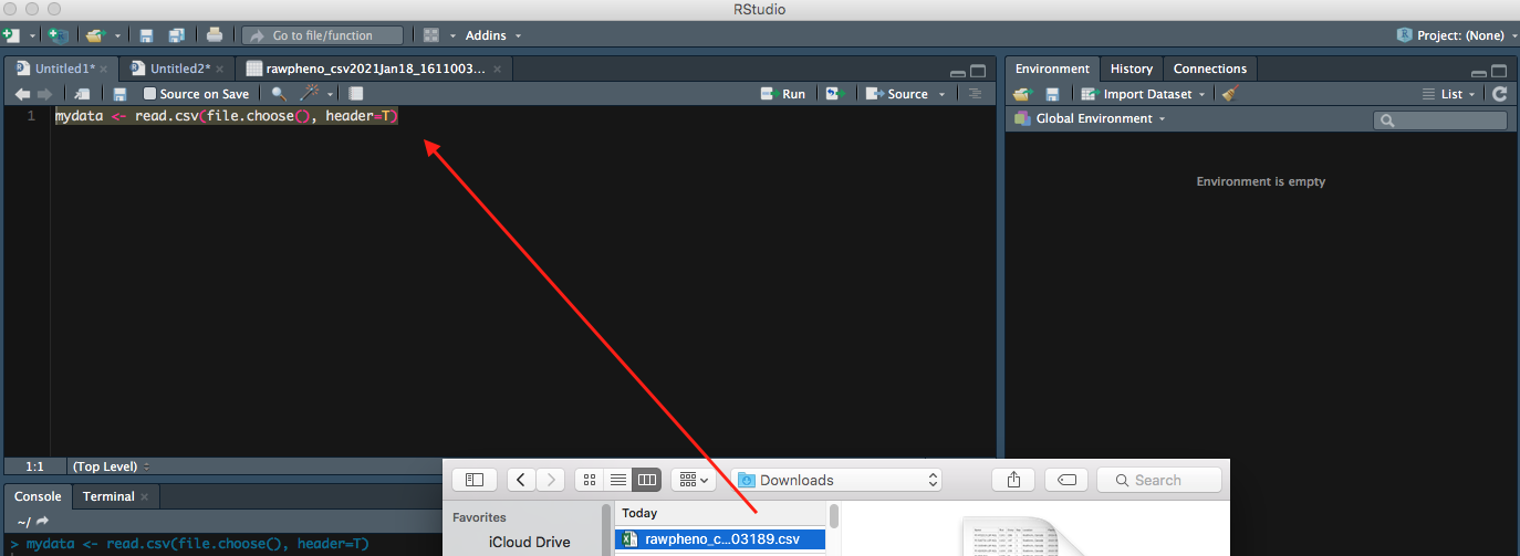
Option 2: Import your read.csv with code
The following command can also be used to import your file. Let us call your file mydata to make it simple.
Step 1
mydata <- read.csv(file.choose(), header=T)
file.choose()command allows a menu poping for you to choose your file, so you donot have to type its full path to find it.header=Teuqals toheader=TRUEmeans you want to keep the first row of your dataset as variable names or headers. Otherwise, you can setheader=FALSE
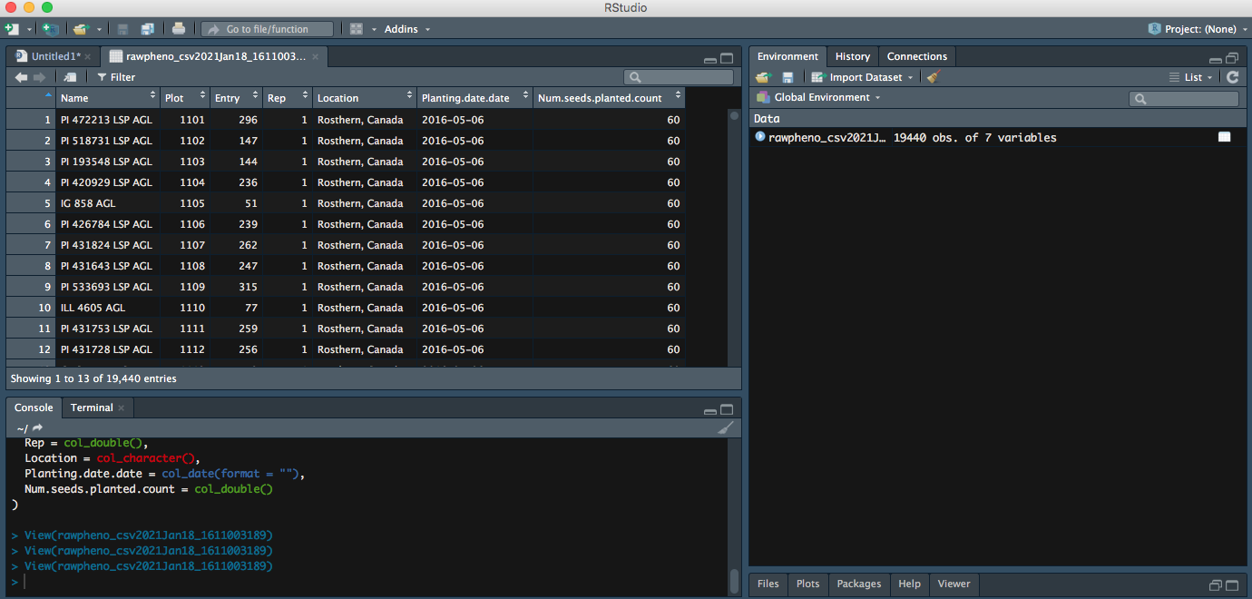
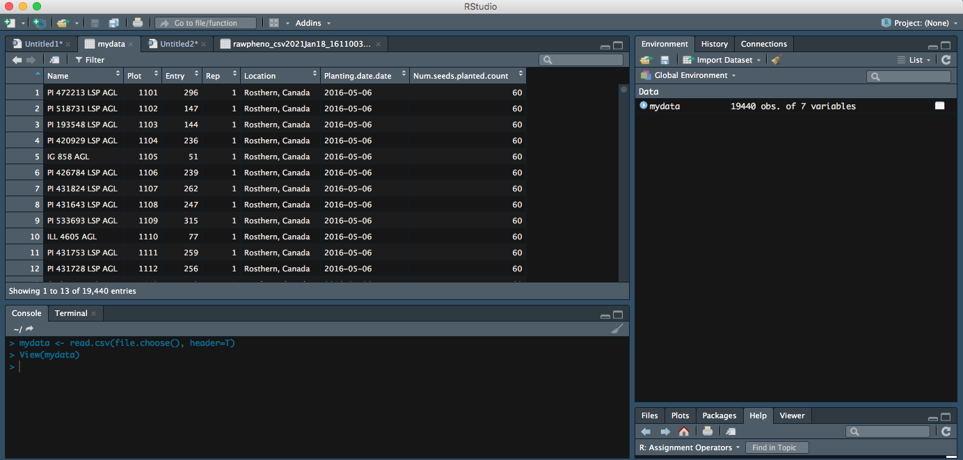
Step 2
Now you can see your entire dataset showing up.
Key Points
read_csv can only be used .csv files.
Tidy data with R
Overview
Teaching: 20 min
Exercises: 20 minQuestions
How to tidy my data after import?
Objectives
Tidy your data for further analysis
Tidy your data
“Tidy datasets are all alike, but every messy dataset is messy in its own way.” –– Hadley Wickham In the previous lesson, you have learned how to import your raw data files into R. But most likely, you will have to tidy up your data after import. In this episode, we are going to learn how to tidy data.
Tidyr Package
Installation
- install.packages(“tidyverse”)
tidyverse core principles:
- Each variable forms a column.
- Each observation forms a row.
- Each type of observational unit forms a table.
6 main verbs
- mutate()
- select()
- filter()
- summarise()
- arrange()
- group by()
Example dataset: DayToFlower.csv
DayToFlower.csv can be downloaded manually from Here
library(tidyverse)
xx <- read_csv("Downloads/DayToFlower.csv")
xx<-na.omit(xx)
yy <- xx %>%
  group_by(Name, Location) %>%
  summarise(Mean_DTF = round(mean(DTF),1)) %>%
  arrange(Location)
yy
## # A tibble: 9 x 3
## # Groups:   Name [3]
##   Name          Location            Mean_DTF
##   <chr>         <chr>                  <dbl>
## 1 CDC Maxim AGL Jessore, Bangladesh     86.7
## 2 ILL 618 AGL   Jessore, Bangladesh     79.3
## 3 Laird AGL     Jessore, Bangladesh     76.8
## 4 CDC Maxim AGL Metaponto, Italy       134.
## 5 ILL 618 AGL   Metaponto, Italy       138.
## 6 Laird AGL     Metaponto, Italy       137.
## 7 CDC Maxim AGL Saskatoon, Canada       52.5
## 8 ILL 618 AGL   Saskatoon, Canada       47
## 9 Laird AGL     Saskatoon, Canada       56.8
yy <- yy %>% spread(key = Location, value = Mean_DTF)
yy
## # A tibble: 3 x 4
## # Groups:   Name [3]
##   Name          `Jessore, Bangladesh` `Metaponto, Italy` `Saskatoon, Canada`
##   <chr>                         <dbl>              <dbl>               <dbl>
## 1 CDC Maxim AGL                  86.7               134.                52.5
## 2 ILL 618 AGL                    79.3               138.                47
## 3 Laird AGL                      76.8               137.                56.8
yy <- yy %>% gather(key = TraitName, value = Value, 2:4)
yy
## # A tibble: 9 x 3
## # Groups:   Name [3]
##   Name          TraitName           Value
##   <chr>         <chr>               <dbl>
## 1 CDC Maxim AGL Jessore, Bangladesh  86.7
## 2 ILL 618 AGL   Jessore, Bangladesh  79.3
## 3 Laird AGL     Jessore, Bangladesh  76.8
## 4 CDC Maxim AGL Metaponto, Italy    134.
## 5 ILL 618 AGL   Metaponto, Italy    138.
## 6 Laird AGL     Metaponto, Italy    137.
## 7 CDC Maxim AGL Saskatoon, Canada    52.5
## 8 ILL 618 AGL   Saskatoon, Canada    47
## 9 Laird AGL     Saskatoon, Canada    56.8
yy <- yy %>% spread(key = Name, value = Value)
yy
## # A tibble: 3 x 4
##   TraitName           `CDC Maxim AGL` `ILL 618 AGL` `Laird AGL`
##   <chr>                         <dbl>         <dbl>       <dbl>
## 1 Jessore, Bangladesh            86.7          79.3        76.8
## 2 Metaponto, Italy              134.          138.        137.
## 3 Saskatoon, Canada              52.5          47          56.8
Key Points
Use the correct verb(s) to rearrange your raw data.
Use xx<-na.omit(xx) command to omit NA values in your raw dataset.
Visualize data in R: Introduction
Overview
Teaching: 20 min
Exercises: 20 minQuestions
How to visualise my data with base plotting?
Objectives
Create various output graphs with basic function
Basic Grahics
We will start with some basic plotting using the base function plot()
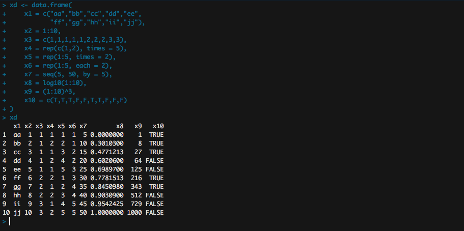
Load a data frame into R
xd <- data.frame(
  x1 = c("aa","bb","cc","dd","ee",
         "ff","gg","hh","ii","jj"),
  x2 = 1:10,
  x3 = c(1,1,1,1,1,2,2,2,3,3),
  x4 = rep(c(1,2), times = 5),
  x5 = rep(1:5, times = 2),
  x6 = rep(1:5, each = 2),
  x7 = seq(5, 50, by = 5),
  x8 = log10(1:10),
  x9 = (1:10)^3,
  x10 = c(T,T,T,F,F,T,T,F,F,F)
)
xd
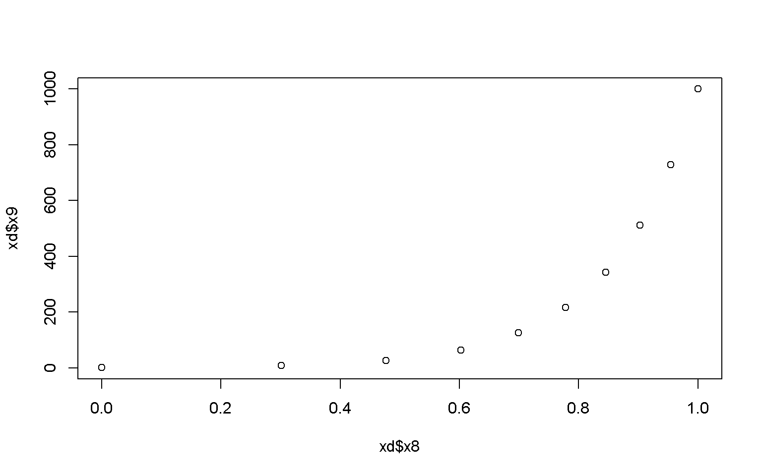
Scatter Plot
A basic scatter plot
plot(x = xd$x8, y = xd$x9)
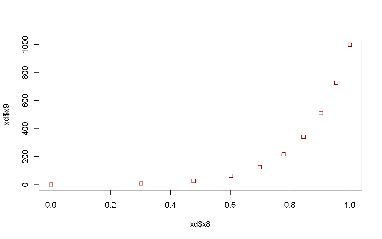
# Adjust color and shape of the points
plot(x = xd$x8, y = xd$x9, col = "darkred", pch = 0)
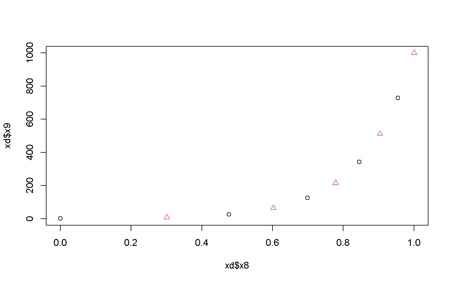
plot(x = xd$x8, y = xd$x9, col = xd$x4, pch = xd$x4)
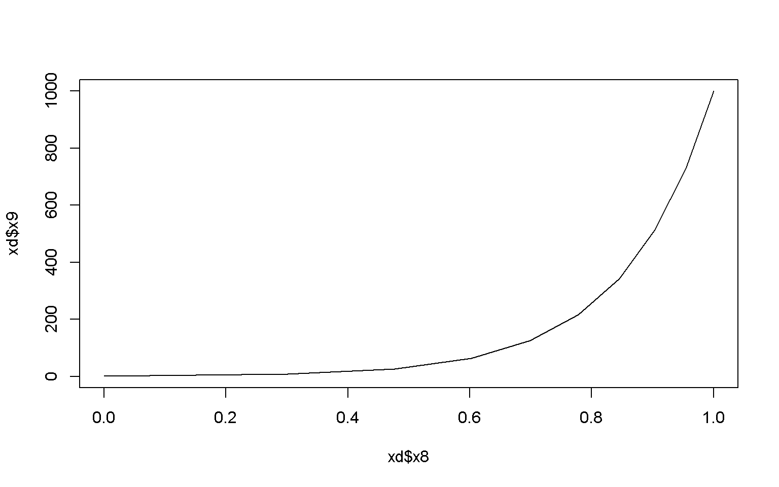
# Adjust plot type
plot(x = xd$x8, y = xd$x9, type = "line")
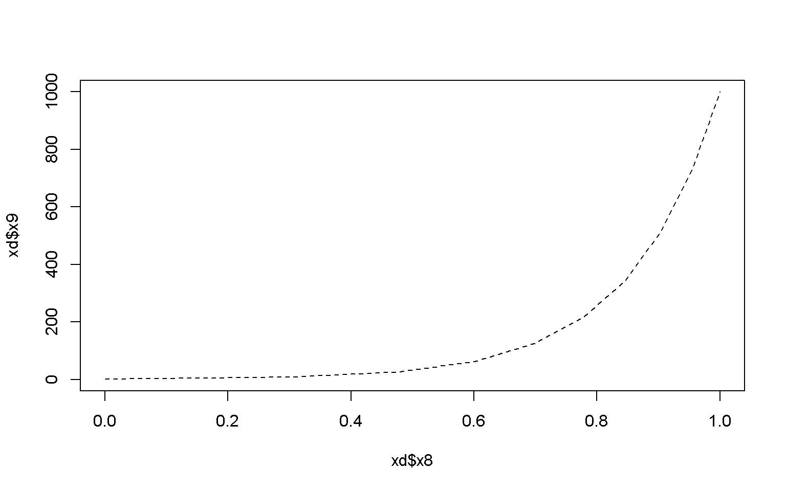
# Adjust linetype
plot(x = xd$x8, y = xd$x9, type = "line", lty = 2)
# Plot lines and points
plot(x = xd$x8, y = xd$x9, type = "both")

Random and normally distributed data to make some more complicated plots:
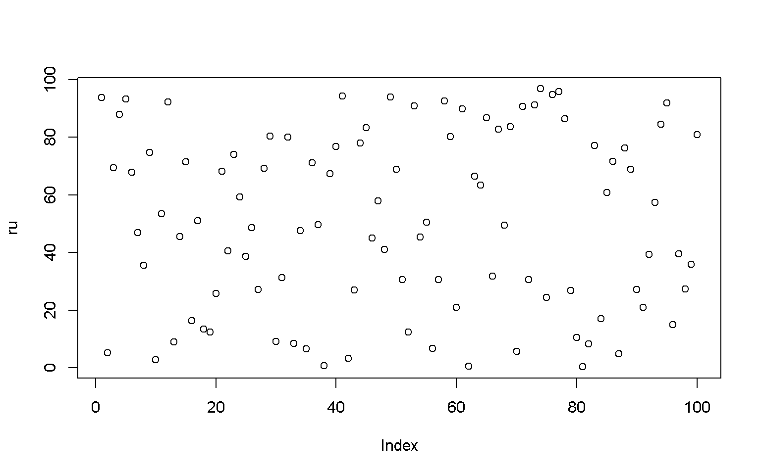
# 100 random uniformly distributed numbers ranging from 0 - 100
ru <- runif(100, min = 0, max = 100)
ru
##   [1] 93.7792722  5.2058264 69.3092606 87.8757695 93.3245922 67.9051869 46.9099487 35.5891664 74.7797008  2.7596956 53.4739481 92.1409410
##  [13]  8.9753618 45.5635354 71.3770539 16.3657328 51.0398228 13.4896518 12.4459450 25.7143970 68.1830481 40.4708243 74.0677972 59.2101567
##  [25] 38.7055322 48.5972122 27.1599634 69.2195419 80.2855715  9.1769648 31.2876002 79.9755078  8.4545997 47.5581250  6.5751686 71.1780116
##  [37] 49.5609812  0.6333086 67.3160462 76.7686795 94.2319493  3.2416026 27.0022919 77.9143718 83.3589595 45.0760499 57.9321392 40.9880216
##  [49] 93.9983372 68.8077655 30.6024296 12.3127829 90.7924286 45.3508709 50.4629388  6.7605921 30.6151922 92.4777183 80.2674523 20.9279168
##  [61] 89.8962399  0.5688416 66.3812347 63.3058209 86.7850871 31.7576001 82.8562194 49.3832795 83.5812209  5.6286126 90.5950977 30.5509194
##  [73] 91.2311482 96.7813272 24.4044569 94.8301130 95.8874951 86.4078381 26.7188237 10.4742400  0.3250012  8.2367471 77.0652131 16.9814142
##  [85] 60.8751291 71.5650256  4.8838718 76.2454340 68.9297517 27.1255990 20.9791733 39.2620779 57.4075861 84.4399911 91.8024827 15.0074634
##  [97] 39.4713569 27.2310661 35.9280103 80.9529896
plot(x = ru)
order(ru)
##   [1]  81  62  38  10  42  87   2  70  35  56  82  33  13  30  80  52  19  18  96  16  84  60  91  75  20  79  43  90  27  98  72  51  57
##  [34]  31  66   8  99  25  92  97  22  48  46  54  14   7  34  26  68  37  55  17  11  93  47  24  85  64  63  39   6  21  50  89  28   3
##  [67]  36  15  86  23   9  88  40  83  44  32  59  29 100  67  45  69  94  78  65   4  61  71  53  73  95  12  58   5   1  49  41  76  77
## [100]  74
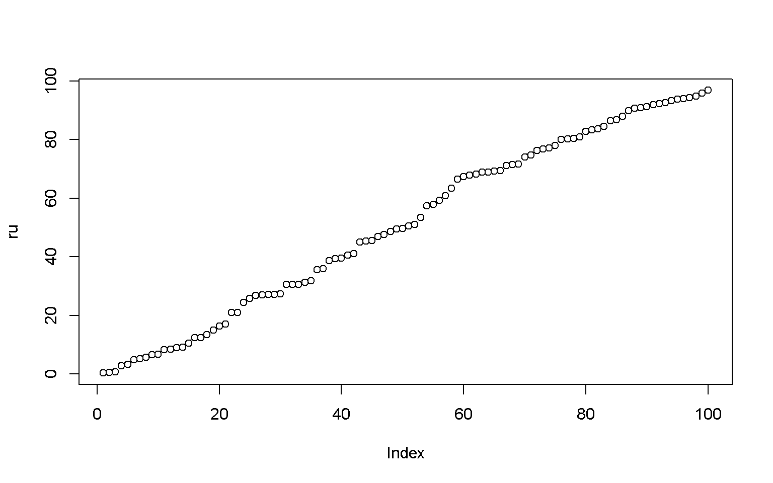
ru<- ru[order(ru)]
ru
##   [1]  0.3250012  0.5688416  0.6333086  2.7596956  3.2416026  4.8838718  5.2058264  5.6286126  6.5751686  6.7605921  8.2367471  8.4545997
##  [13]  8.9753618  9.1769648 10.4742400 12.3127829 12.4459450 13.4896518 15.0074634 16.3657328 16.9814142 20.9279168 20.9791733 24.4044569
##  [25] 25.7143970 26.7188237 27.0022919 27.1255990 27.1599634 27.2310661 30.5509194 30.6024296 30.6151922 31.2876002 31.7576001 35.5891664
##  [37] 35.9280103 38.7055322 39.2620779 39.4713569 40.4708243 40.9880216 45.0760499 45.3508709 45.5635354 46.9099487 47.5581250 48.5972122
##  [49] 49.3832795 49.5609812 50.4629388 51.0398228 53.4739481 57.4075861 57.9321392 59.2101567 60.8751291 63.3058209 66.3812347 67.3160462
##  [61] 67.9051869 68.1830481 68.8077655 68.9297517 69.2195419 69.3092606 71.1780116 71.3770539 71.5650256 74.0677972 74.7797008 76.2454340
##  [73] 76.7686795 77.0652131 77.9143718 79.9755078 80.2674523 80.2855715 80.9529896 82.8562194 83.3589595 83.5812209 84.4399911 86.4078381
##  [85] 86.7850871 87.8757695 89.8962399 90.5950977 90.7924286 91.2311482 91.8024827 92.1409410 92.4777183 93.3245922 93.7792722 93.9983372
##  [97] 94.2319493 94.8301130 95.8874951 96.7813272
plot(x = ru)
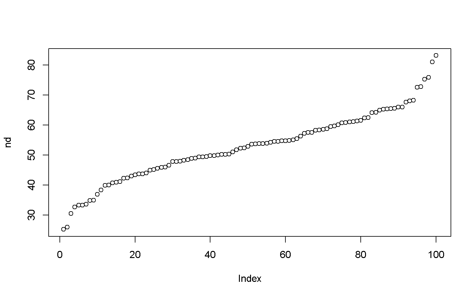
# 100 normally distributed numbers with a mean of 50 and sd of 10
nd <- rnorm(100, mean = 50, sd = 10)
nd
##   [1] 38.40931 54.50517 61.00758 48.24371 55.05703 50.19036 75.92284 65.39284 58.75954 42.96810 45.87521 58.25970 47.82696 45.19008
##  [15] 54.57716 43.44305 67.67423 55.49420 42.37655 68.21933 49.80417 54.71856 33.31593 34.93320 46.63470 53.88502 48.86226 47.84021
##  [29] 65.98524 61.40776 40.74877 26.02507 30.57845 51.05247 43.76863 83.17006 25.25972 51.80369 54.21798 68.06235 53.69070 34.84286
##  [43] 64.18536 60.73534 58.38647 60.15617 53.86052 33.32625 49.78303 54.79121 42.29689 44.92490 57.54842 49.39659 65.47622 62.40080
##  [57] 58.58921 57.18908 48.48429 40.02540 49.49290 47.99492 59.49275 52.43222 64.25810 75.30217 72.62295 33.67732 81.02630 61.60500
##  [71] 61.17238 36.94567 32.65669 60.83920 54.88921 50.03472 66.01779 40.95968 65.58695 56.29101 48.98033 39.95974 50.33351 57.50313
##  [85] 44.06732 59.69696 45.56645 41.10511 46.04440 43.69505 64.95305 52.92210 53.65435 62.51068 52.27743 65.31862 72.85238 53.81886
##  [99] 49.44123 50.25871
nd <- nd[order(nd)]
nd
##   [1] 25.25972 26.02507 30.57845 32.65669 33.31593 33.32625 33.67732 34.84286 34.93320 36.94567 38.40931 39.95974 40.02540 40.74877
##  [15] 40.95968 41.10511 42.29689 42.37655 42.96810 43.44305 43.69505 43.76863 44.06732 44.92490 45.19008 45.56645 45.87521 46.04440
##  [29] 46.63470 47.82696 47.84021 47.99492 48.24371 48.48429 48.86226 48.98033 49.39659 49.44123 49.49290 49.78303 49.80417 50.03472
##  [43] 50.19036 50.25871 50.33351 51.05247 51.80369 52.27743 52.43222 52.92210 53.65435 53.69070 53.81886 53.86052 53.88502 54.21798
##  [57] 54.50517 54.57716 54.71856 54.79121 54.88921 55.05703 55.49420 56.29101 57.18908 57.50313 57.54842 58.25970 58.38647 58.58921
##  [71] 58.75954 59.49275 59.69696 60.15617 60.73534 60.83920 61.00758 61.17238 61.40776 61.60500 62.40080 62.51068 64.18536 64.25810
##  [85] 64.95305 65.31862 65.39284 65.47622 65.58695 65.98524 66.01779 67.67423 68.06235 68.21933 72.62295 72.85238 75.30217 75.92284
##  [99] 81.02630 83.17006
plot(x = nd)
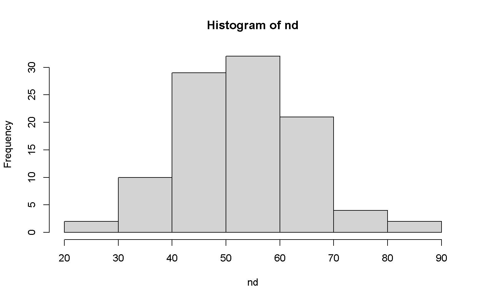
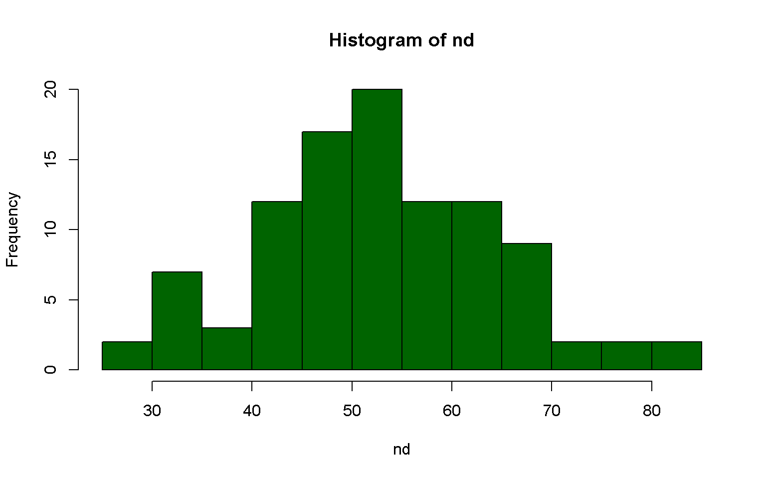
Histogram
hist(x = nd)
hist(nd, breaks = 20, col = "darkgreen")
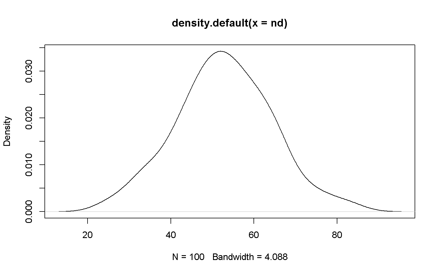
plot(x = density(nd))
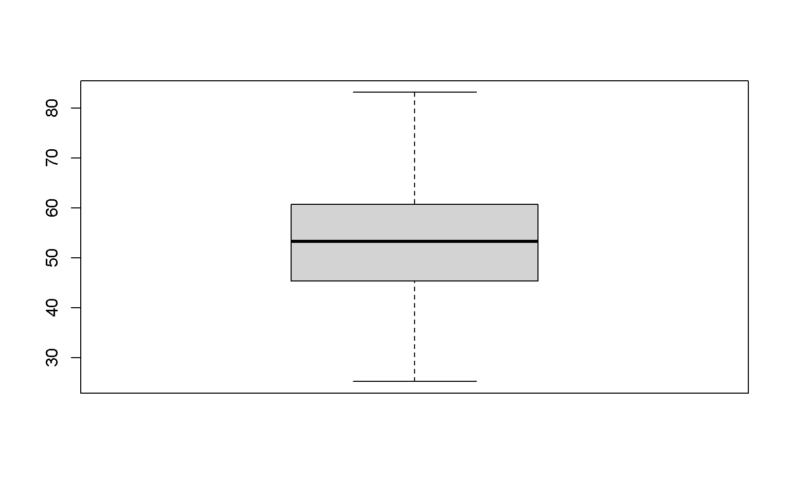
Boxplot
boxplot(x = nd)
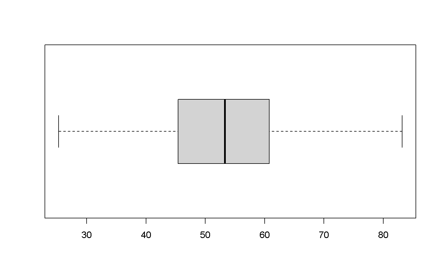
boxplot(x = nd, horizontal = T)
Key Points
Customize your graphs to make them more visually appealling.
Visualize data in R: ggplot2 package and more
Overview
Teaching: 20 min
Exercises: 30 minQuestions
How to plot data with ggplot2?
Objectives
Visuallize your data with ggplot2.
ggplot2 package
Compare to basic plots, ggplot2 package provides better visually appealing plots. ggplot2 package needs to be installed before use.
Install
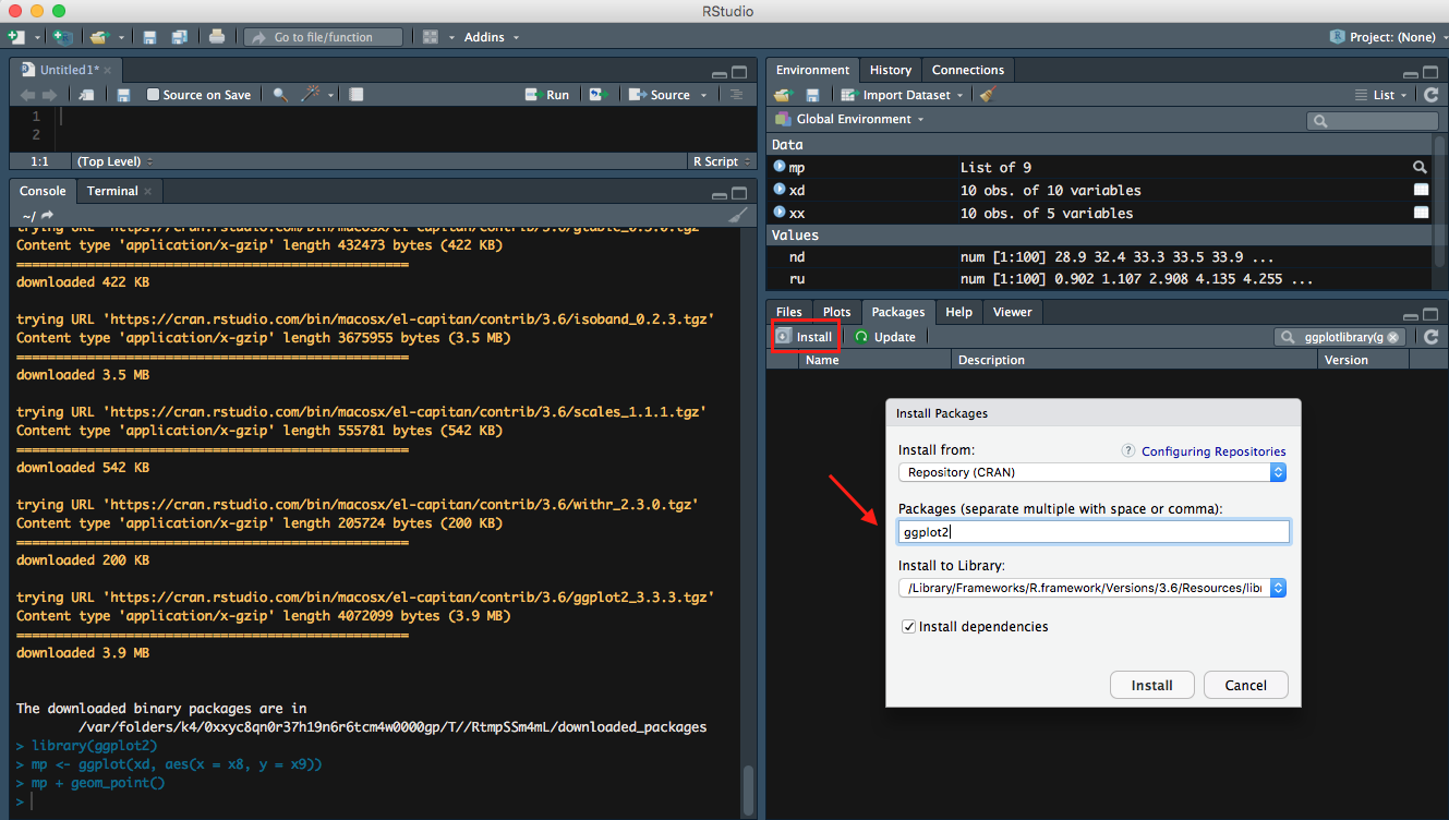
click on Packages tab, select on Install, then search ggplo2 under Packages to install ggplots2.
- ggplot2 is one of the core packeages from
Tidyverse, so you may already downloaded it from previous lesson.
Useful Resources
- Data Visualization with ggplot2 Cheat Sheet
- ggplot2 part of the tidyverse
- ggplot2
- How to make any plot in ggplot2?
- Graphics in R with ggplot2
Points
library(ggplot2)
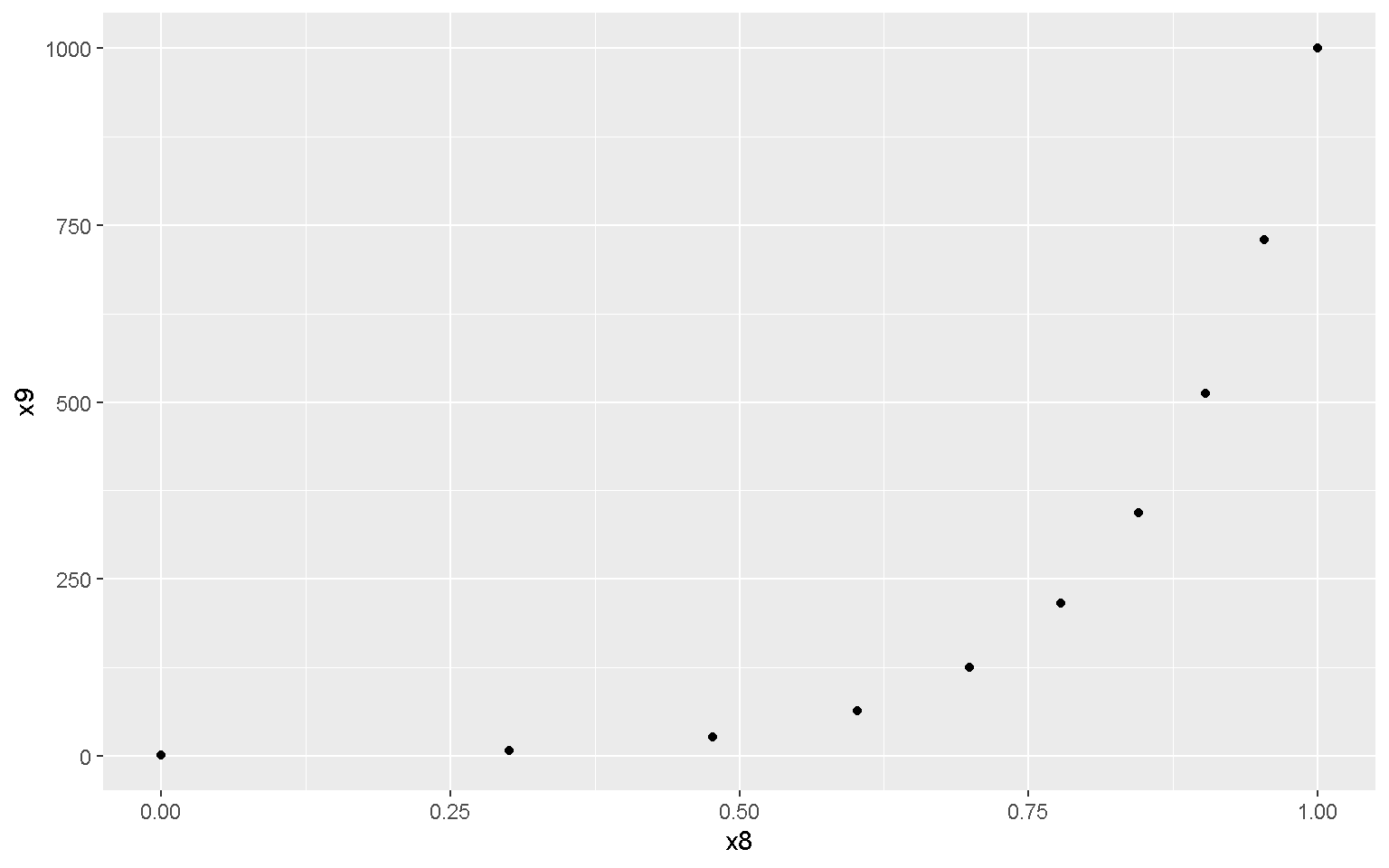
mp <- ggplot(xd, aes(x = x8, y = x9))
mp + geom_point()
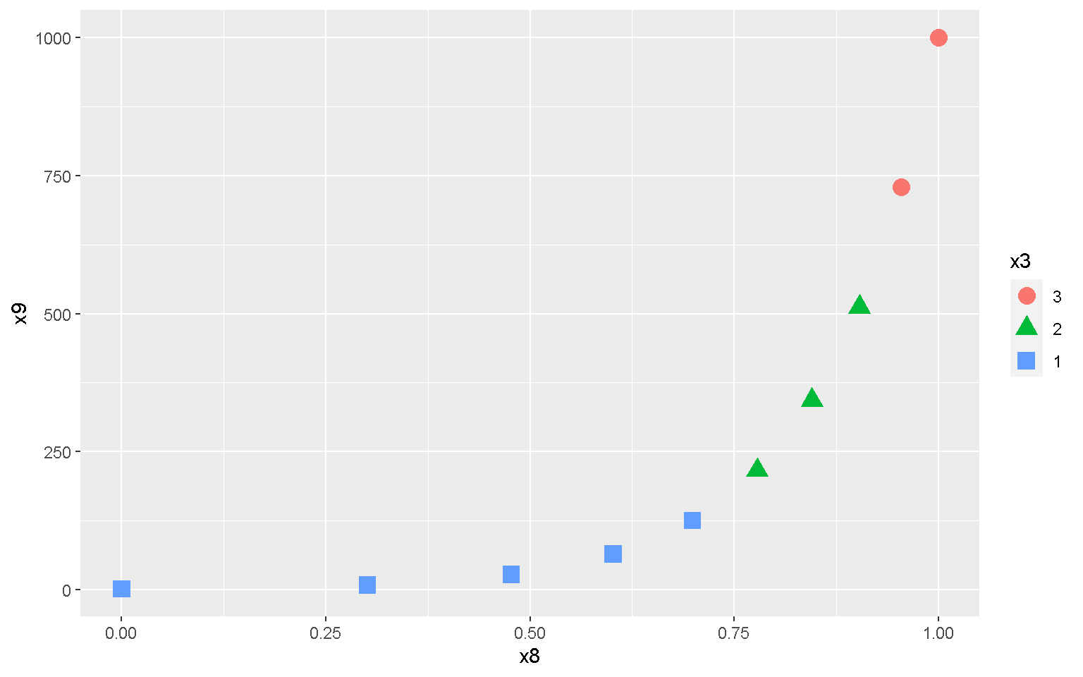
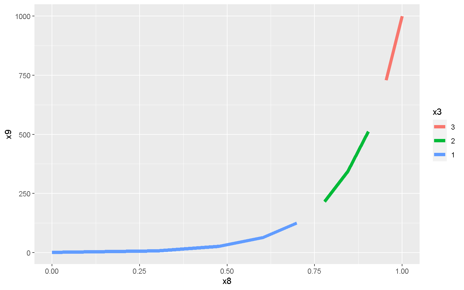
mp + geom_point(aes(color = x3, shape = x3), size = 4)
Lines
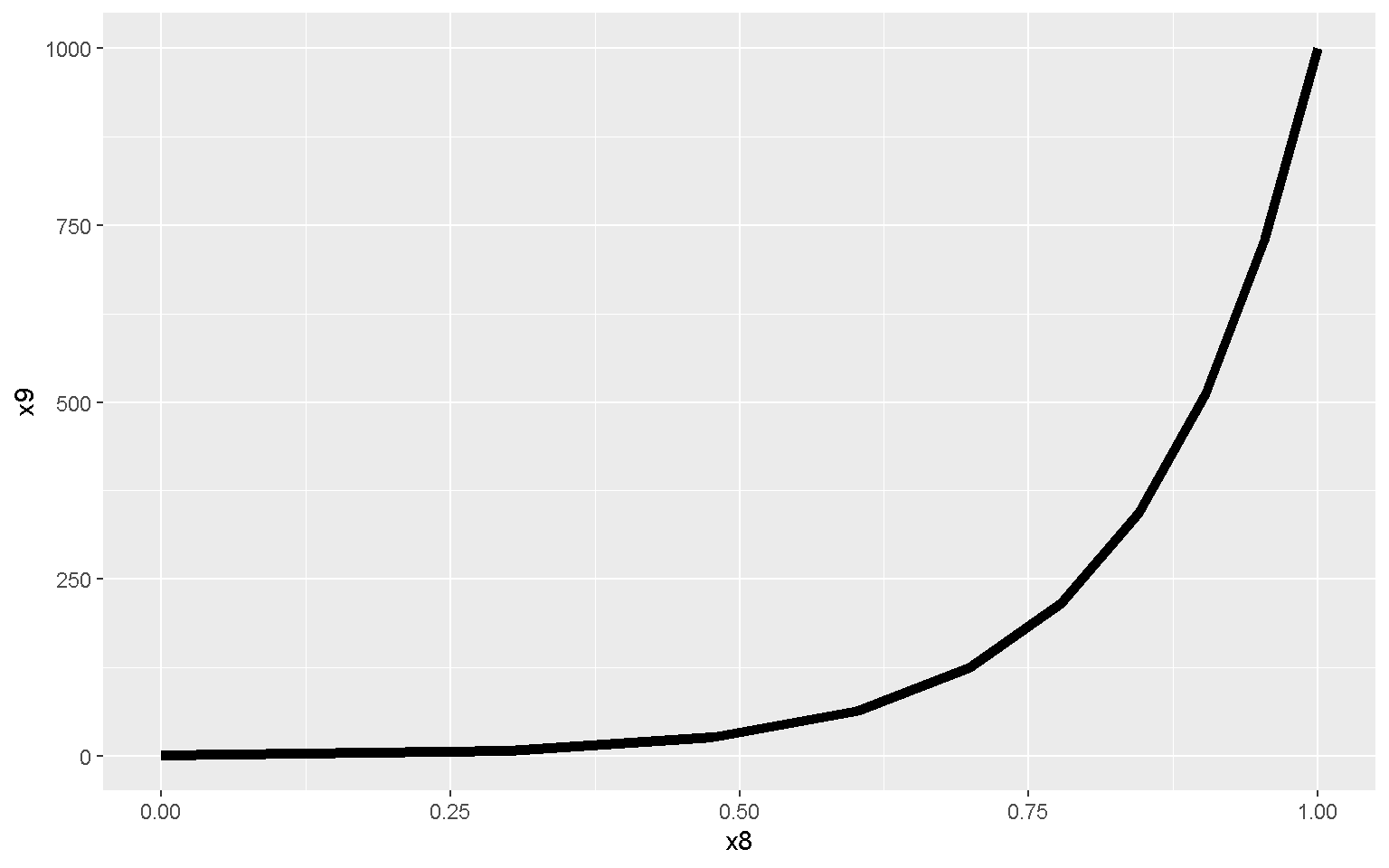
mp + geom_line(size = 2)
mp + geom_line(aes(color = x3), size = 2)
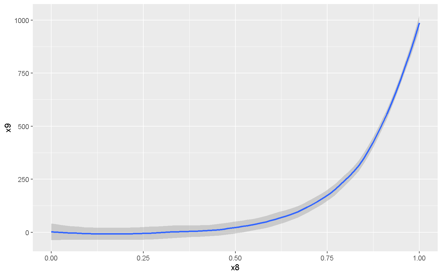
Smoothed Conditional Means
mp + geom_smooth(method = "loess")
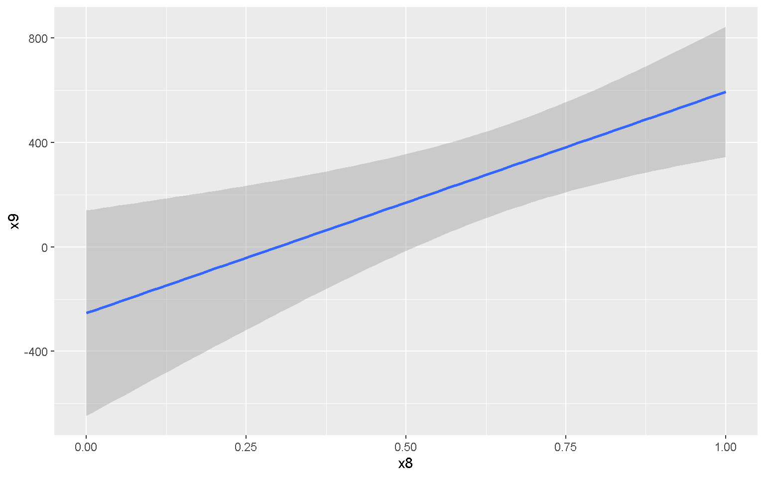
mp + geom_smooth(method = "lm")
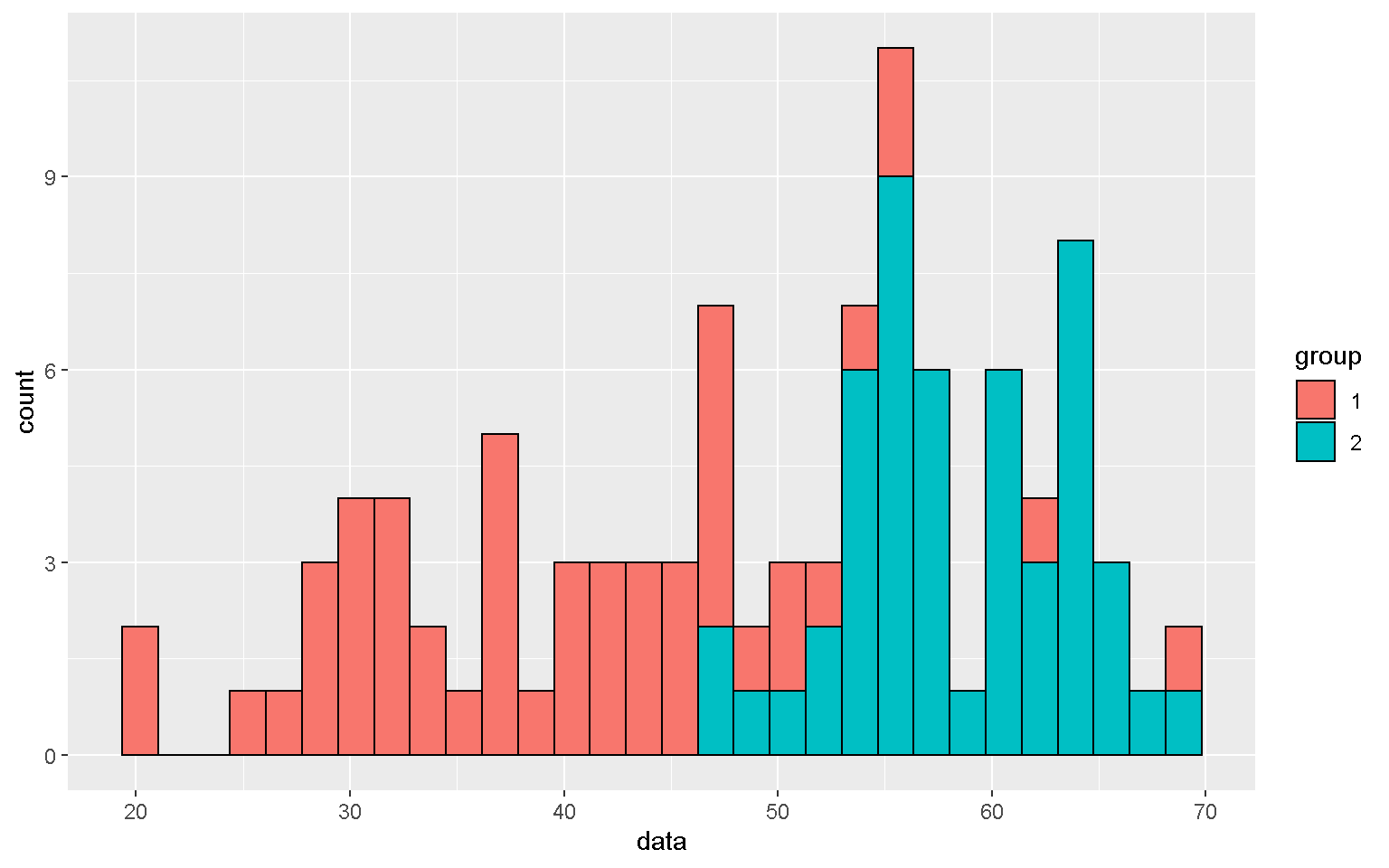
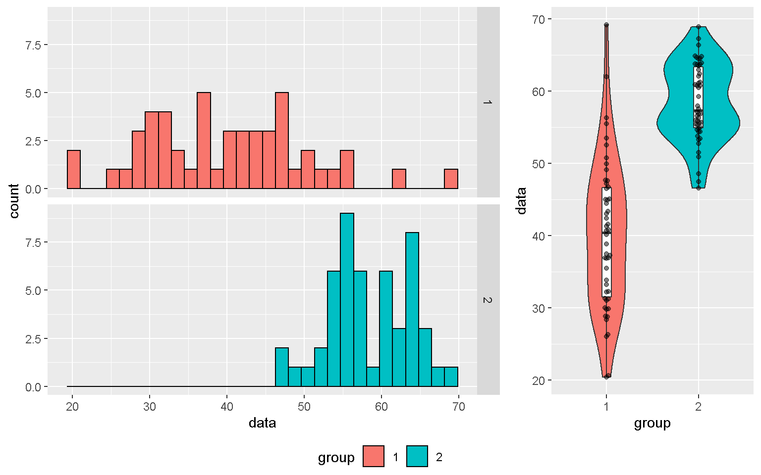
Histogram
xx <- data.frame(data = c(rnorm(50, mean = 40, sd = 10),
rnorm(50, mean = 60, sd = 5)),
group = factor(rep(1:2, each = 50)),
label = c("Label1", rep(NA, 49), "Label2", rep(NA, 49)))
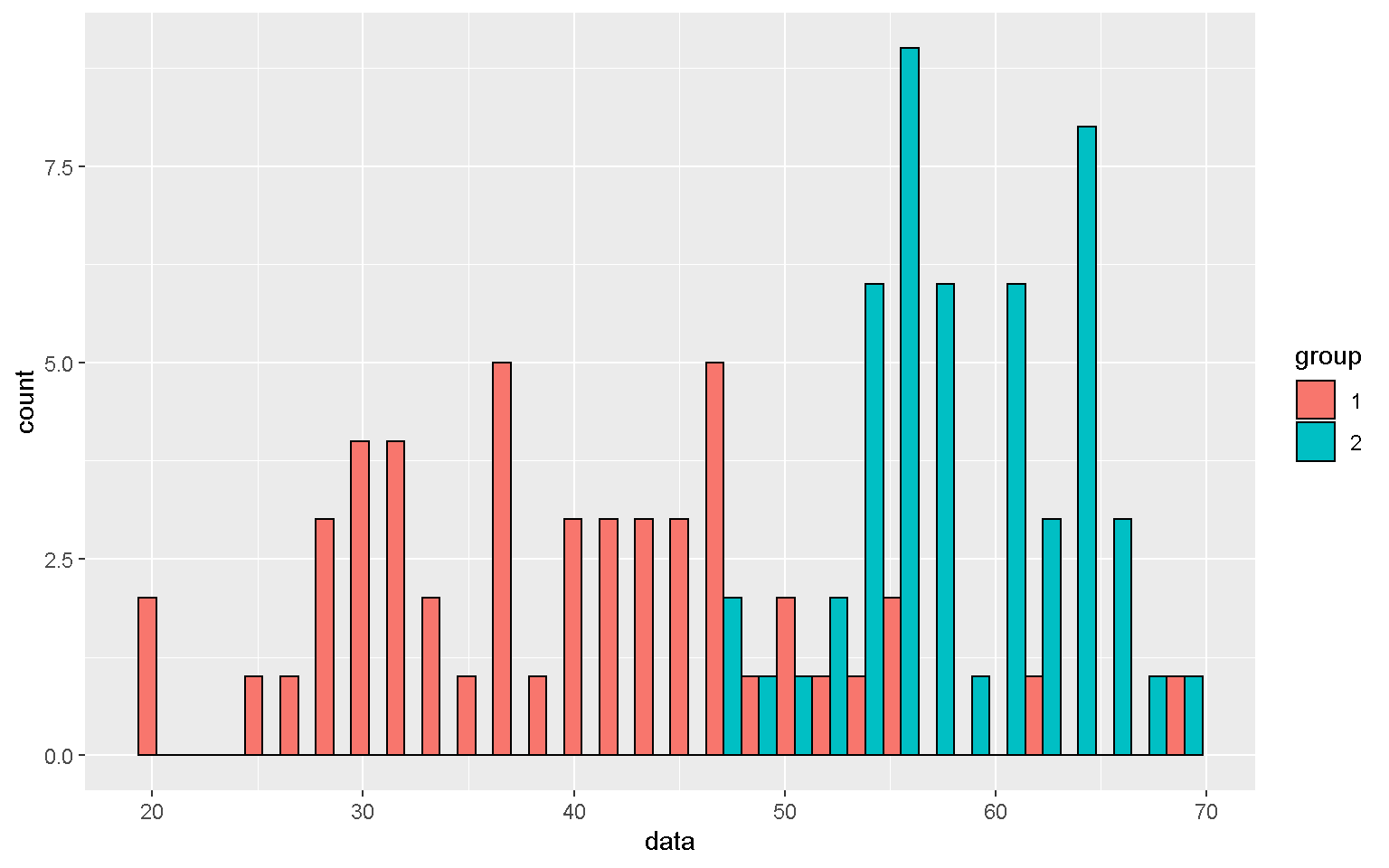
mp <- ggplot(xx, aes(x = data, fill = group))
mp + geom_histogram(color = "black")
mp + geom_histogram(color = "black", position = "dodge")
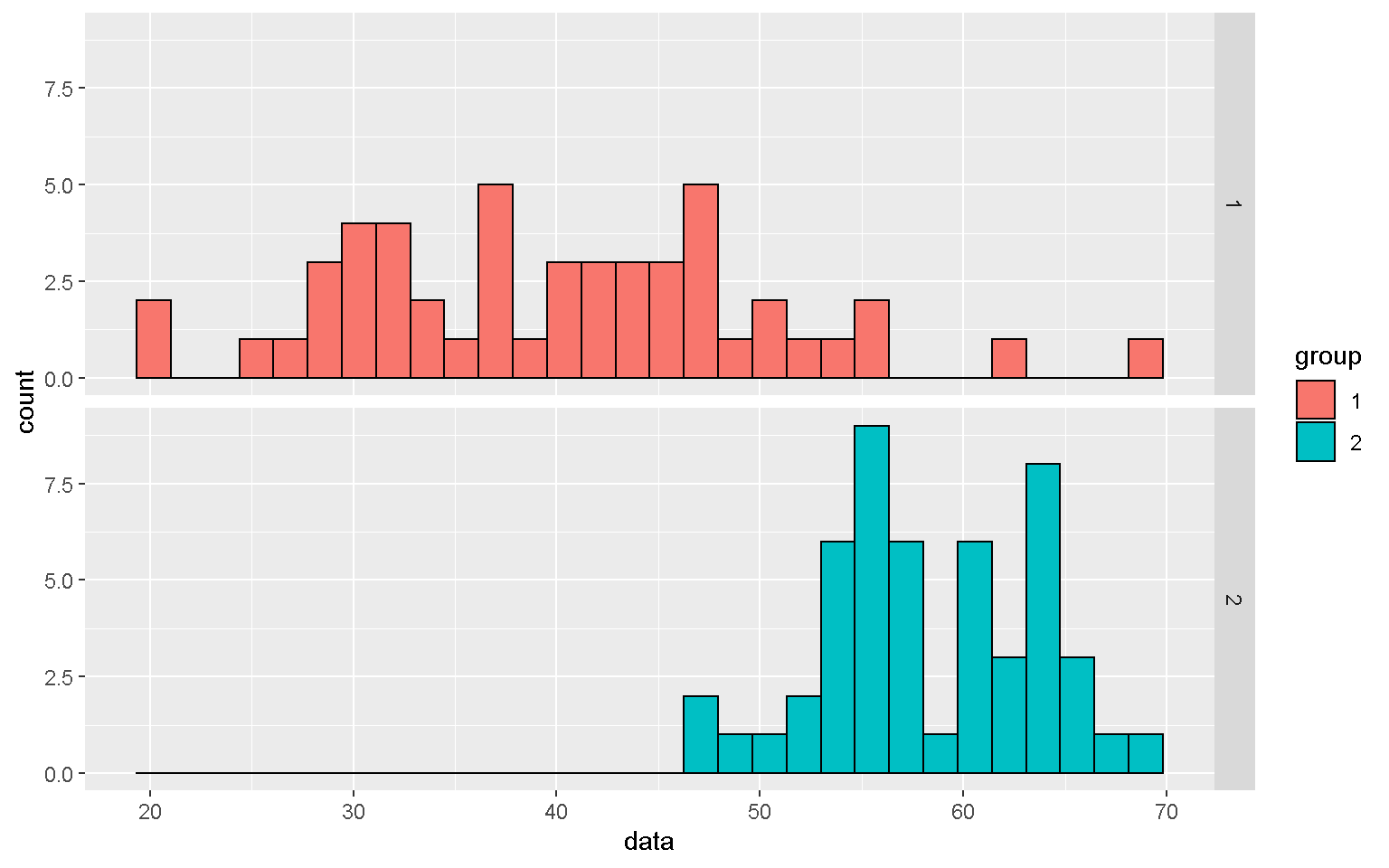
mp1 <- mp + geom_histogram(color = "black") + facet_grid(group~.)
mp1
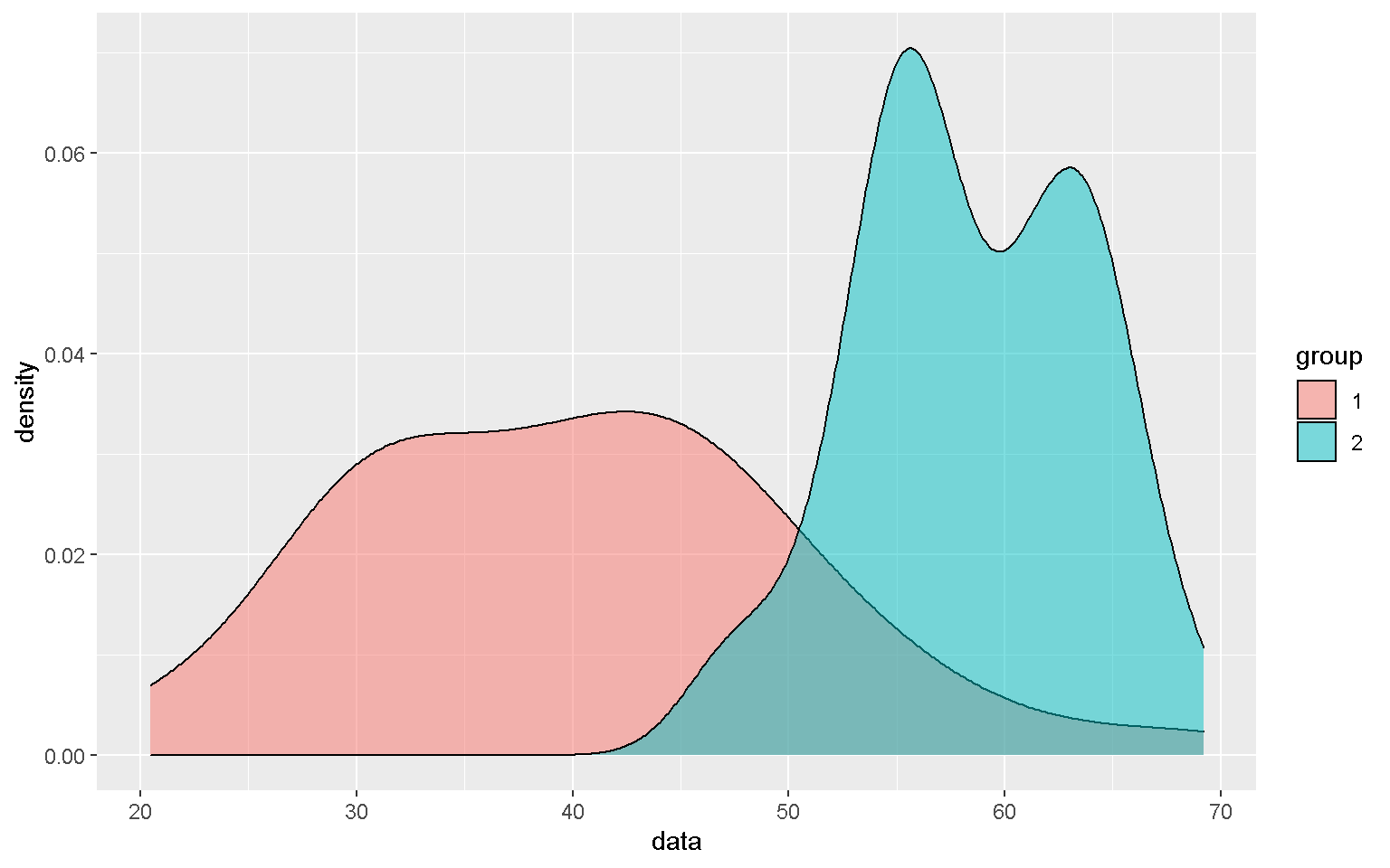
Smoothed density estimates
mp + geom_density(alpha = 0.5)
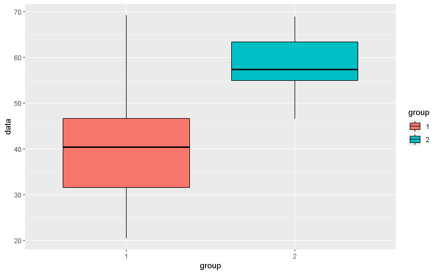
Boxplot
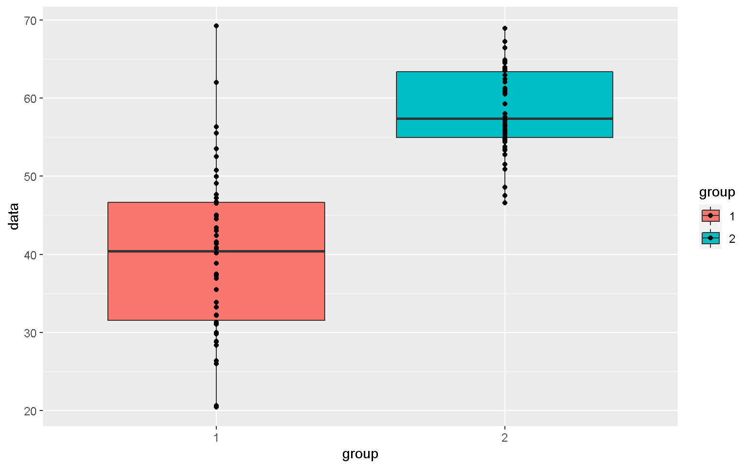
mp <- ggplot(xx, aes(x = group, y = data, fill = group))
mp + geom_boxplot(color = "black")
mp + geom_boxplot() + geom_point()
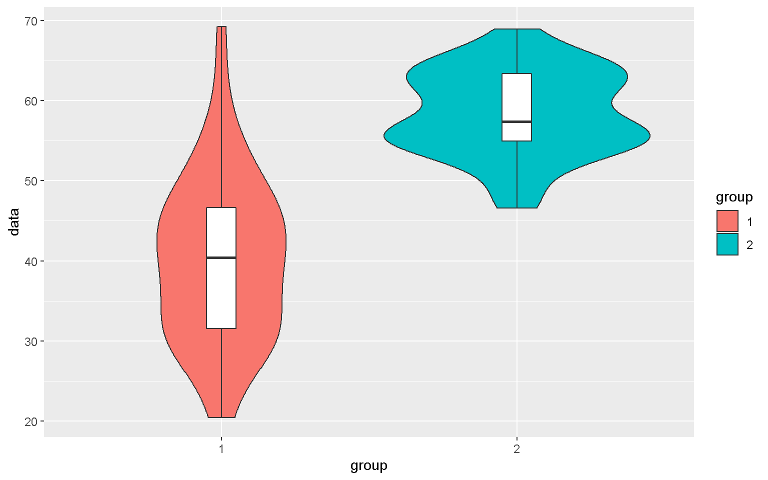
Violin Plot
mp + geom_violin() + geom_boxplot(width = 0.1, fill = "white")
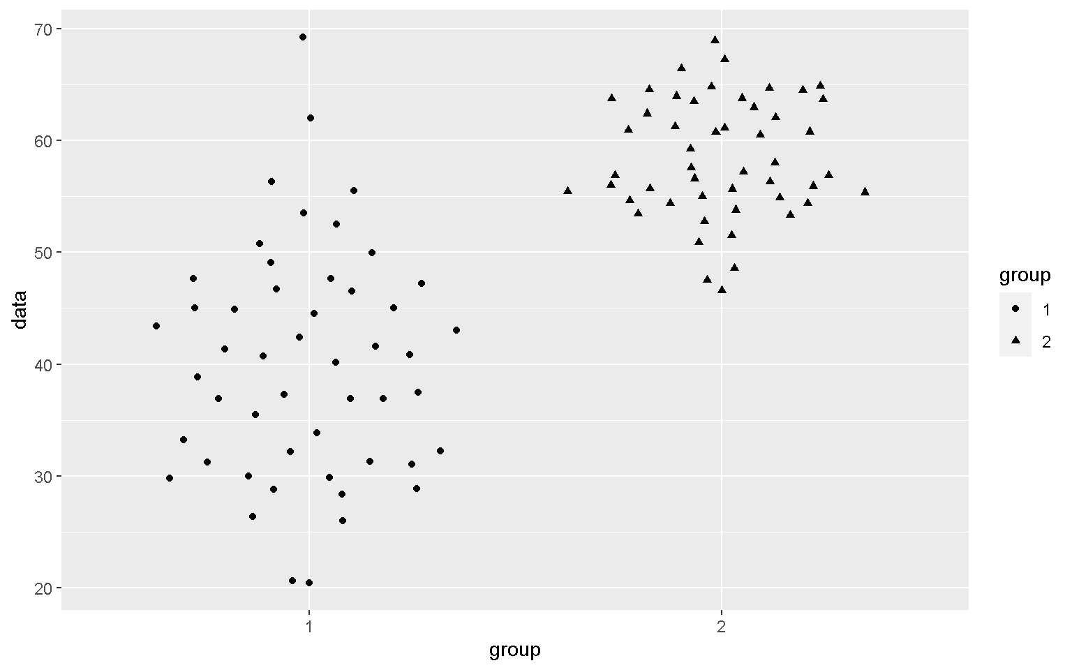
library(ggbeeswarm)
mp + geom_quasirandom()
Additional packages such as ggbeeswarm and ggrepel also contain useful functions to add to the functionality of ggplot2

mp + geom_quasirandom(aes(shape = group))
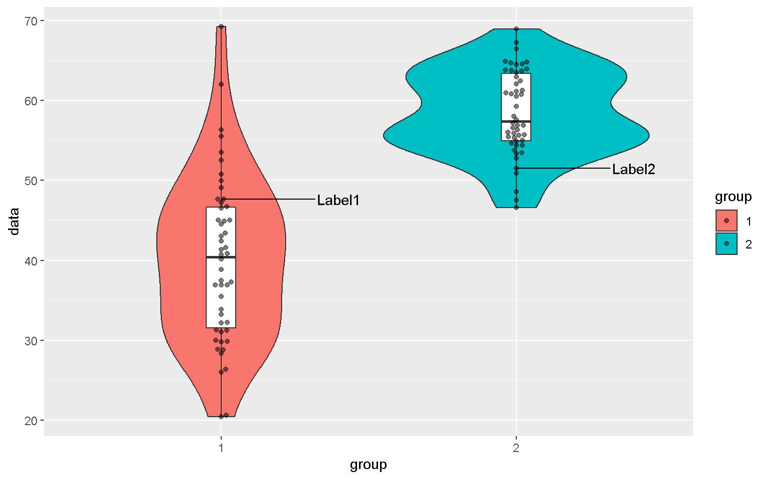
mp2 <- mp + geom_violin() +
  geom_boxplot(width = 0.1, fill = "white") +
  geom_beeswarm(alpha = 0.5)
library(ggrepel)
mp2 + geom_text_repel(aes(label = label), nudge_x = 0.4)
library(ggpubr)
ggarrange(mp1, mp2, ncol = 2, widths = c(2,1),
          common.legend = T, legend = "bottom")
Key Points
Remember to load your ggplot2 library before writing your code
Find the best graph meets your need
Export your data from R
Overview
Teaching: 20 min
Exercises: 20 minQuestions
How to export my tidy file?
Objectives
Export a tidy file from R
Work.table Command to export your data from R
We are aiming to output the .csv file we have tidied from last episode.
#Save the exported file in Downloads
setwd("Downloads")
#Read your data from Downloads
xx <- read_csv("Downloads/DayToFlower.csv")
xx <- read_xlsx("Downloads/DayToFlower.xlsx", sheet = "DayToFlower")
xx<-na.omit(xx)
yy <- xx %>%
  group_by(Name, Location) %>%
  summarise(Mean_DTF = round(mean(DTF),1)) %>%
  arrange(Location)
yy
#Your coad
yy <- yy %>% spread(key = Location, value = Mean_DTF)
yy
yy <- yy %>% gather(key = TraitName, value = Value, 2:4)
yy
yy <- yy %>% spread(key = Name, value = Value)
yy
write.table(yy,file="DataToExport.csv", sep=",")
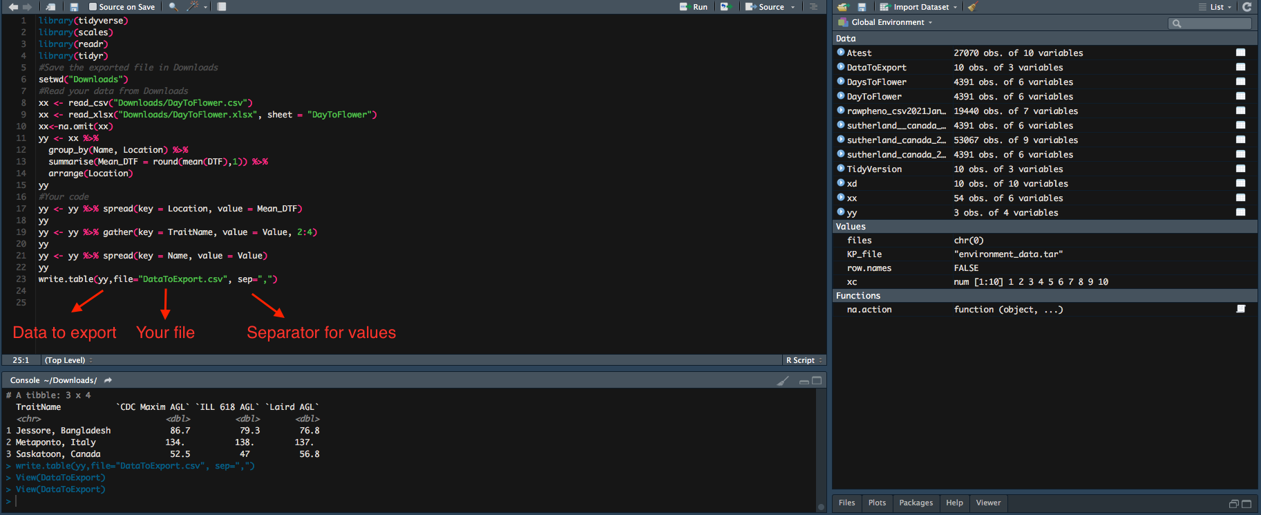
Now your DataToExport.csv is saved in Downloads.
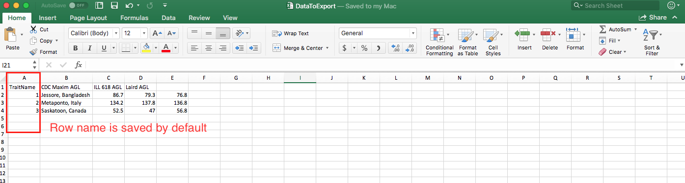
To remove row name
write.table(yy,file="DataToExport.csv", row.names=F, sep=",")
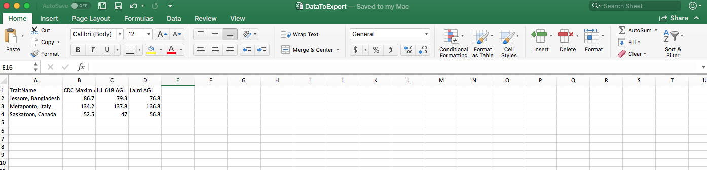
- The old file is overwritten by the new one, so you only get one
DataToExport.csv. - Exported file can be saved in different formats through change of the separator. Check Export Data from R for details.
Key Points
Make sure to indicate where you would like to see the exported file.
Set row.names=F to remove unwanted row names while exporting your file.