Visualize data in R: Introduction
Overview
Teaching: 20 min
Exercises: 20 minQuestions
How to visualise my data with base plotting?
Objectives
Create various output graphs with basic function
Basic Grahics
We will start with some basic plotting using the base function plot()
Load a data frame into R
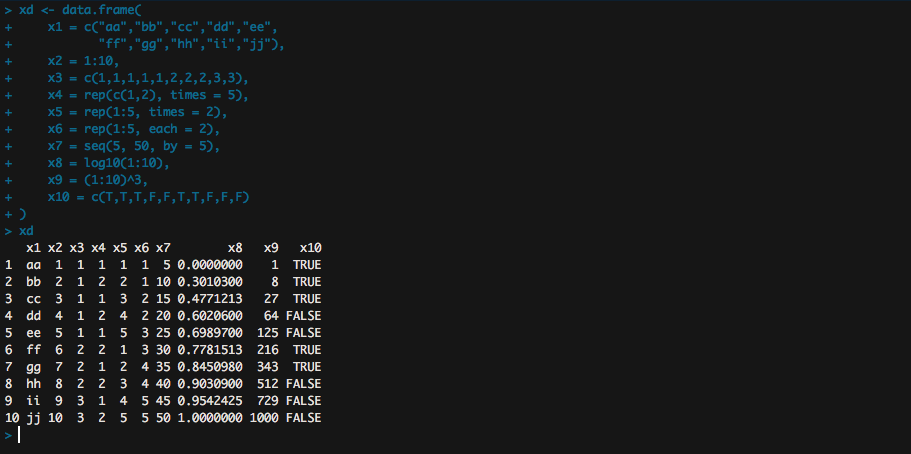
xd <- data.frame(
  x1 = c("aa","bb","cc","dd","ee",
         "ff","gg","hh","ii","jj"),
  x2 = 1:10,
  x3 = c(1,1,1,1,1,2,2,2,3,3),
  x4 = rep(c(1,2), times = 5),
  x5 = rep(1:5, times = 2),
  x6 = rep(1:5, each = 2),
  x7 = seq(5, 50, by = 5),
  x8 = log10(1:10),
  x9 = (1:10)^3,
  x10 = c(T,T,T,F,F,T,T,F,F,F)
)
xd
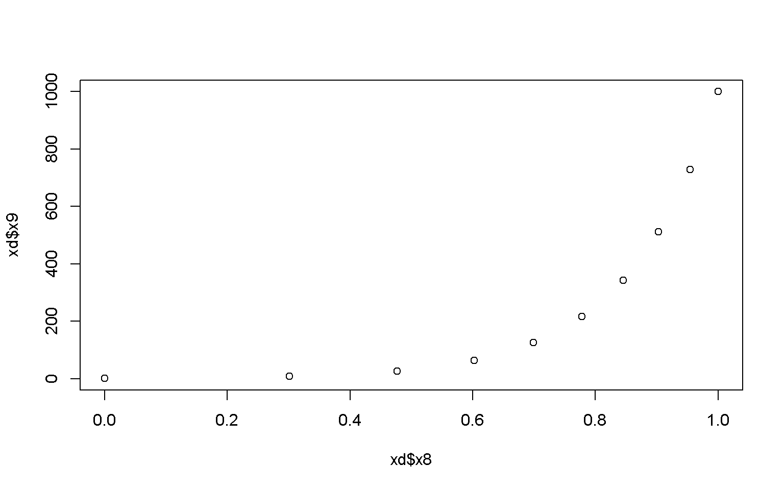
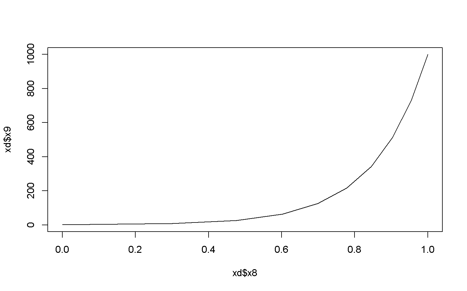
Scatter Plot
A basic scatter plot
plot(x = xd$x8, y = xd$x9)
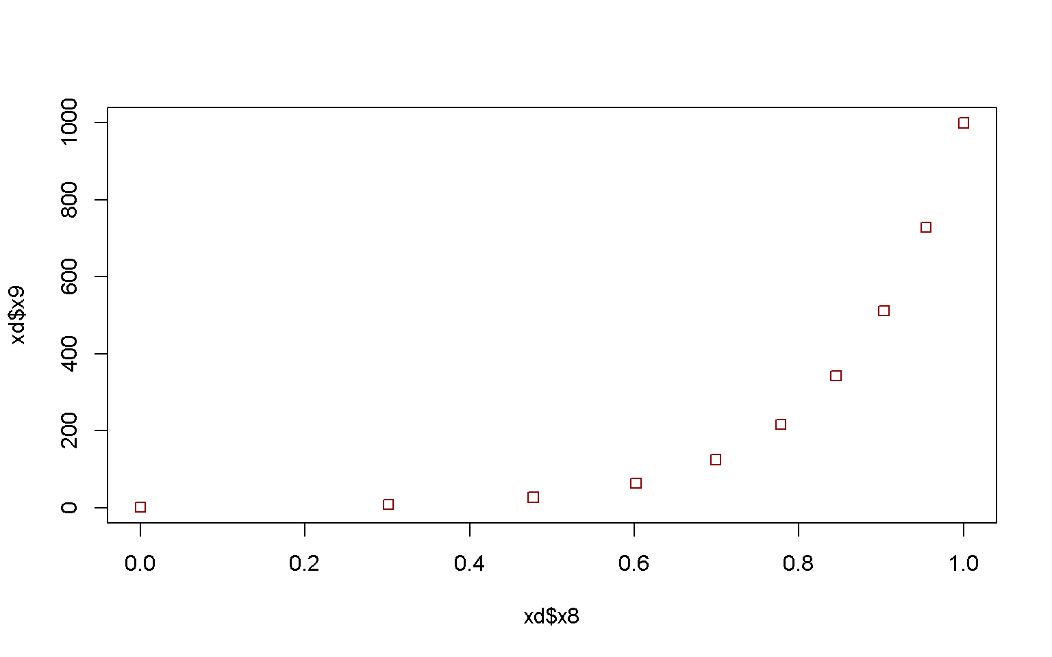
# Adjust color and shape of the points
plot(x = xd$x8, y = xd$x9, col = "darkred", pch = 0)
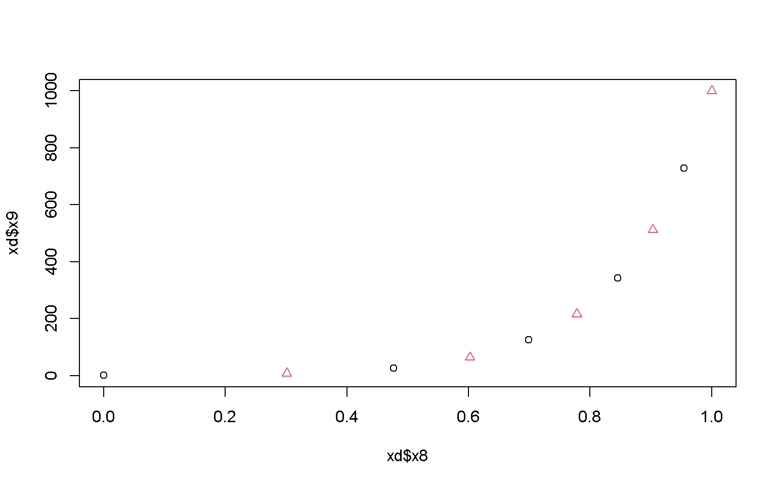
plot(x = xd$x8, y = xd$x9, col = xd$x4, pch = xd$x4)
# Adjust plot type
plot(x = xd$x8, y = xd$x9, type = "line")
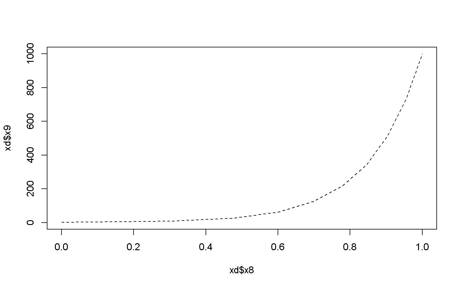
# Adjust linetype
plot(x = xd$x8, y = xd$x9, type = "line", lty = 2)
# Plot lines and points
plot(x = xd$x8, y = xd$x9, type = "both")

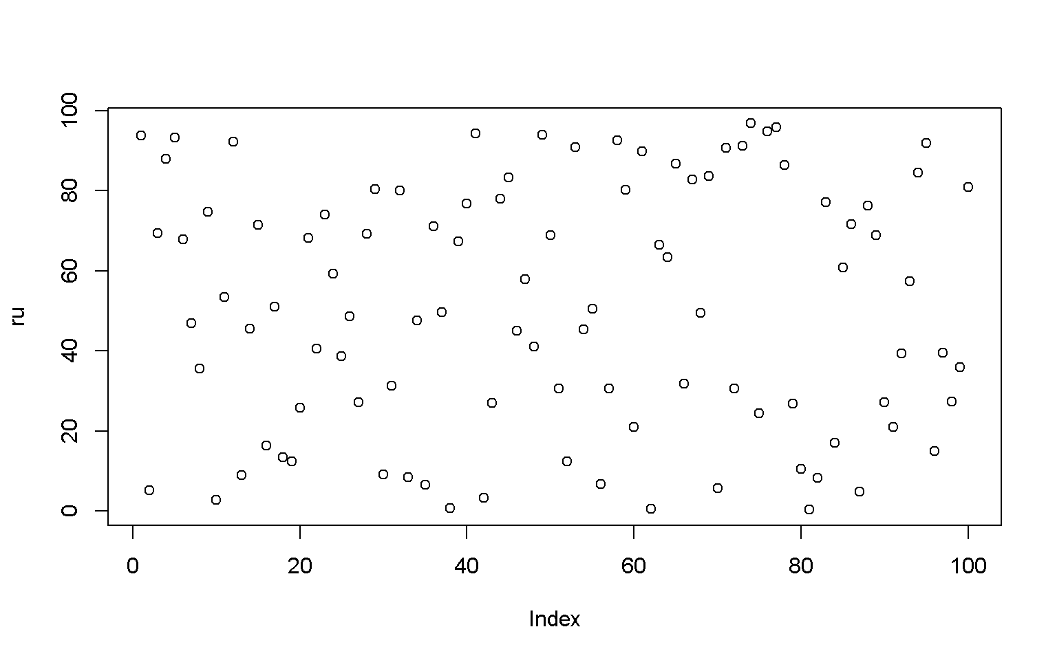
Random and normally distributed data to make some more complicated plots:
# 100 random uniformly distributed numbers ranging from 0 - 100
ru <- runif(100, min = 0, max = 100)
ru
##   [1] 93.7792722  5.2058264 69.3092606 87.8757695 93.3245922 67.9051869 46.9099487 35.5891664 74.7797008  2.7596956 53.4739481 92.1409410
##  [13]  8.9753618 45.5635354 71.3770539 16.3657328 51.0398228 13.4896518 12.4459450 25.7143970 68.1830481 40.4708243 74.0677972 59.2101567
##  [25] 38.7055322 48.5972122 27.1599634 69.2195419 80.2855715  9.1769648 31.2876002 79.9755078  8.4545997 47.5581250  6.5751686 71.1780116
##  [37] 49.5609812  0.6333086 67.3160462 76.7686795 94.2319493  3.2416026 27.0022919 77.9143718 83.3589595 45.0760499 57.9321392 40.9880216
##  [49] 93.9983372 68.8077655 30.6024296 12.3127829 90.7924286 45.3508709 50.4629388  6.7605921 30.6151922 92.4777183 80.2674523 20.9279168
##  [61] 89.8962399  0.5688416 66.3812347 63.3058209 86.7850871 31.7576001 82.8562194 49.3832795 83.5812209  5.6286126 90.5950977 30.5509194
##  [73] 91.2311482 96.7813272 24.4044569 94.8301130 95.8874951 86.4078381 26.7188237 10.4742400  0.3250012  8.2367471 77.0652131 16.9814142
##  [85] 60.8751291 71.5650256  4.8838718 76.2454340 68.9297517 27.1255990 20.9791733 39.2620779 57.4075861 84.4399911 91.8024827 15.0074634
##  [97] 39.4713569 27.2310661 35.9280103 80.9529896
plot(x = ru)
order(ru)
##   [1]  81  62  38  10  42  87   2  70  35  56  82  33  13  30  80  52  19  18  96  16  84  60  91  75  20  79  43  90  27  98  72  51  57
##  [34]  31  66   8  99  25  92  97  22  48  46  54  14   7  34  26  68  37  55  17  11  93  47  24  85  64  63  39   6  21  50  89  28   3
##  [67]  36  15  86  23   9  88  40  83  44  32  59  29 100  67  45  69  94  78  65   4  61  71  53  73  95  12  58   5   1  49  41  76  77
## [100]  74
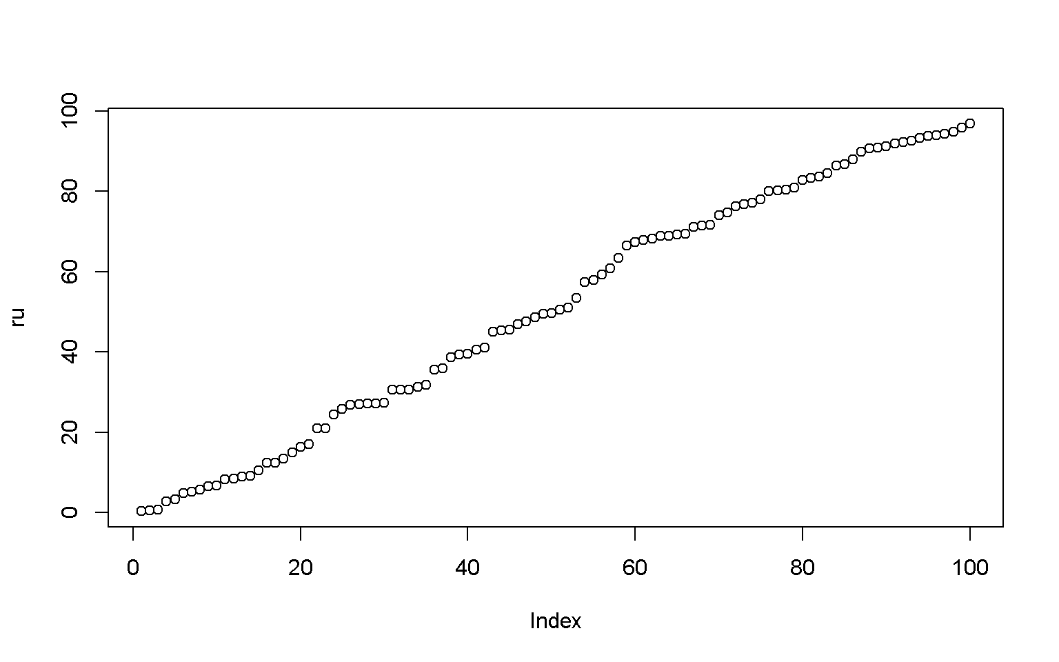
ru<- ru[order(ru)]
ru
##   [1]  0.3250012  0.5688416  0.6333086  2.7596956  3.2416026  4.8838718  5.2058264  5.6286126  6.5751686  6.7605921  8.2367471  8.4545997
##  [13]  8.9753618  9.1769648 10.4742400 12.3127829 12.4459450 13.4896518 15.0074634 16.3657328 16.9814142 20.9279168 20.9791733 24.4044569
##  [25] 25.7143970 26.7188237 27.0022919 27.1255990 27.1599634 27.2310661 30.5509194 30.6024296 30.6151922 31.2876002 31.7576001 35.5891664
##  [37] 35.9280103 38.7055322 39.2620779 39.4713569 40.4708243 40.9880216 45.0760499 45.3508709 45.5635354 46.9099487 47.5581250 48.5972122
##  [49] 49.3832795 49.5609812 50.4629388 51.0398228 53.4739481 57.4075861 57.9321392 59.2101567 60.8751291 63.3058209 66.3812347 67.3160462
##  [61] 67.9051869 68.1830481 68.8077655 68.9297517 69.2195419 69.3092606 71.1780116 71.3770539 71.5650256 74.0677972 74.7797008 76.2454340
##  [73] 76.7686795 77.0652131 77.9143718 79.9755078 80.2674523 80.2855715 80.9529896 82.8562194 83.3589595 83.5812209 84.4399911 86.4078381
##  [85] 86.7850871 87.8757695 89.8962399 90.5950977 90.7924286 91.2311482 91.8024827 92.1409410 92.4777183 93.3245922 93.7792722 93.9983372
##  [97] 94.2319493 94.8301130 95.8874951 96.7813272
plot(x = ru)
# 100 normally distributed numbers with a mean of 50 and sd of 10
nd <- rnorm(100, mean = 50, sd = 10)
nd
##   [1] 38.40931 54.50517 61.00758 48.24371 55.05703 50.19036 75.92284 65.39284 58.75954 42.96810 45.87521 58.25970 47.82696 45.19008
##  [15] 54.57716 43.44305 67.67423 55.49420 42.37655 68.21933 49.80417 54.71856 33.31593 34.93320 46.63470 53.88502 48.86226 47.84021
##  [29] 65.98524 61.40776 40.74877 26.02507 30.57845 51.05247 43.76863 83.17006 25.25972 51.80369 54.21798 68.06235 53.69070 34.84286
##  [43] 64.18536 60.73534 58.38647 60.15617 53.86052 33.32625 49.78303 54.79121 42.29689 44.92490 57.54842 49.39659 65.47622 62.40080
##  [57] 58.58921 57.18908 48.48429 40.02540 49.49290 47.99492 59.49275 52.43222 64.25810 75.30217 72.62295 33.67732 81.02630 61.60500
##  [71] 61.17238 36.94567 32.65669 60.83920 54.88921 50.03472 66.01779 40.95968 65.58695 56.29101 48.98033 39.95974 50.33351 57.50313
##  [85] 44.06732 59.69696 45.56645 41.10511 46.04440 43.69505 64.95305 52.92210 53.65435 62.51068 52.27743 65.31862 72.85238 53.81886
##  [99] 49.44123 50.25871
nd <- nd[order(nd)]
nd
##   [1] 25.25972 26.02507 30.57845 32.65669 33.31593 33.32625 33.67732 34.84286 34.93320 36.94567 38.40931 39.95974 40.02540 40.74877
##  [15] 40.95968 41.10511 42.29689 42.37655 42.96810 43.44305 43.69505 43.76863 44.06732 44.92490 45.19008 45.56645 45.87521 46.04440
##  [29] 46.63470 47.82696 47.84021 47.99492 48.24371 48.48429 48.86226 48.98033 49.39659 49.44123 49.49290 49.78303 49.80417 50.03472
##  [43] 50.19036 50.25871 50.33351 51.05247 51.80369 52.27743 52.43222 52.92210 53.65435 53.69070 53.81886 53.86052 53.88502 54.21798
##  [57] 54.50517 54.57716 54.71856 54.79121 54.88921 55.05703 55.49420 56.29101 57.18908 57.50313 57.54842 58.25970 58.38647 58.58921
##  [71] 58.75954 59.49275 59.69696 60.15617 60.73534 60.83920 61.00758 61.17238 61.40776 61.60500 62.40080 62.51068 64.18536 64.25810
##  [85] 64.95305 65.31862 65.39284 65.47622 65.58695 65.98524 66.01779 67.67423 68.06235 68.21933 72.62295 72.85238 75.30217 75.92284
##  [99] 81.02630 83.17006
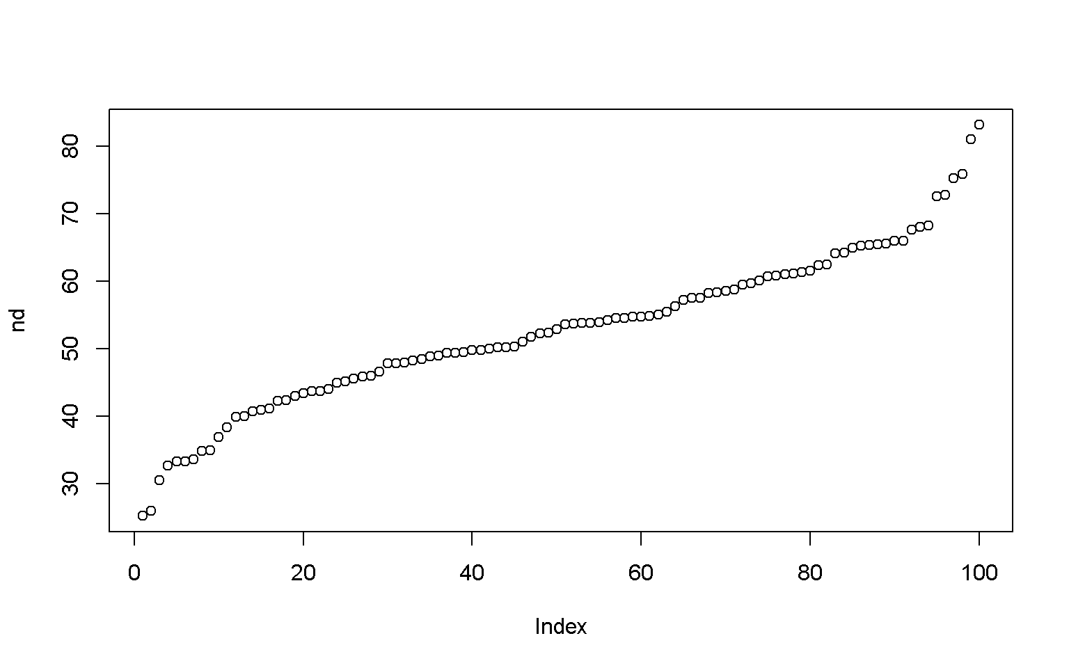
plot(x = nd)
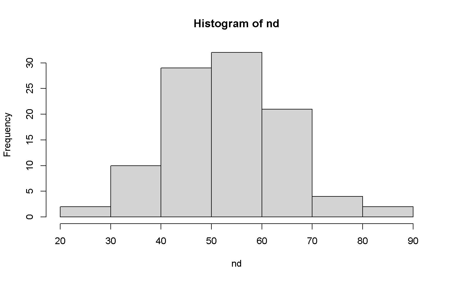
Histogram
hist(x = nd)
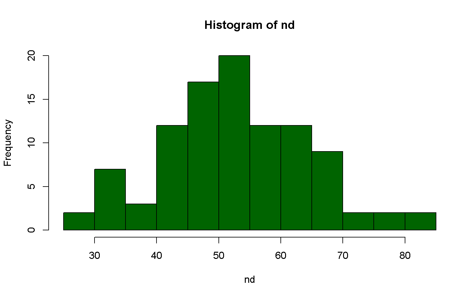
hist(nd, breaks = 20, col = "darkgreen")
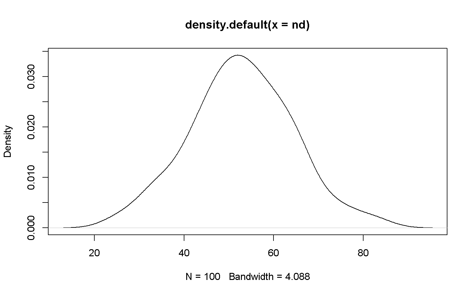
plot(x = density(nd))
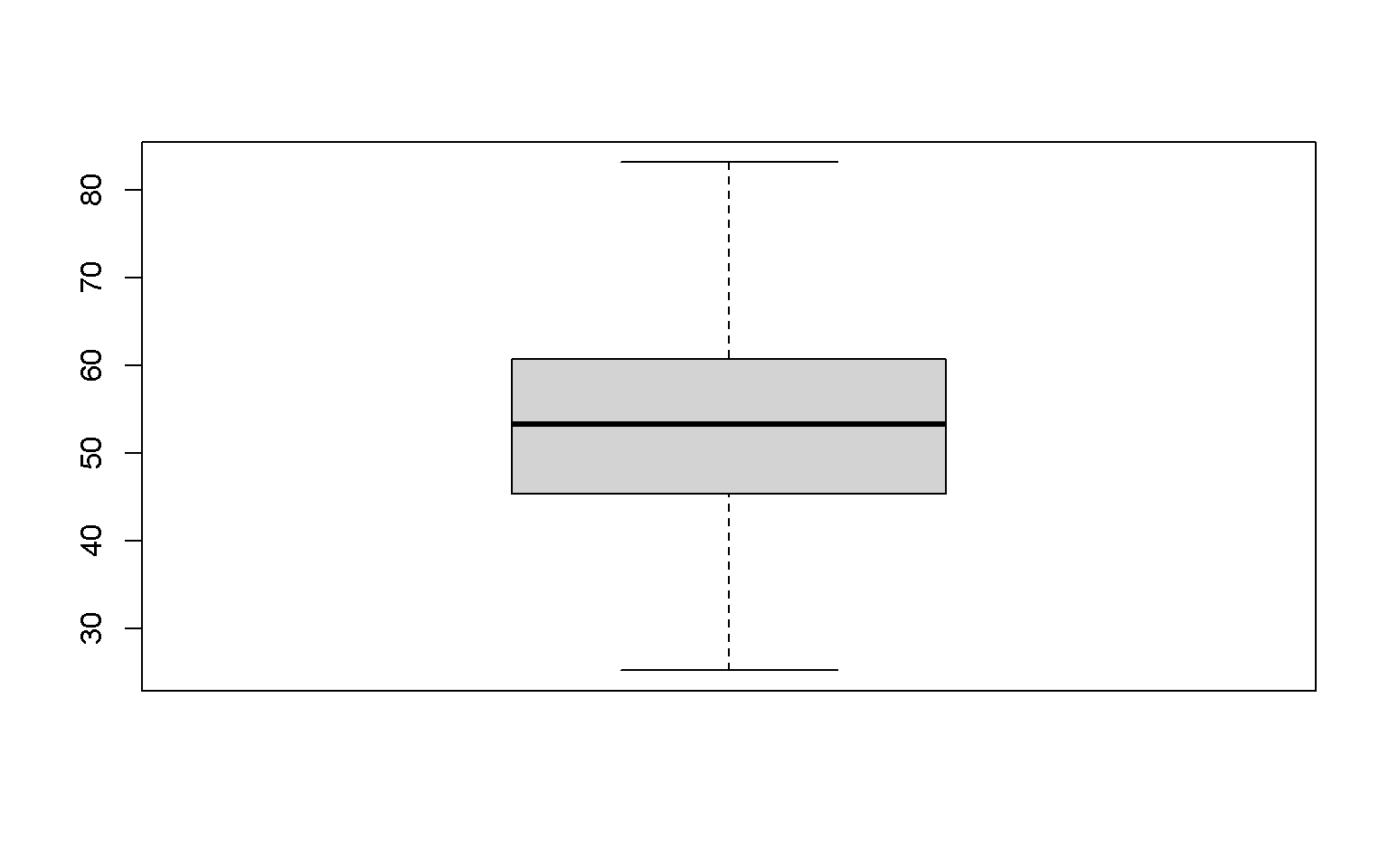
Boxplot
boxplot(x = nd)
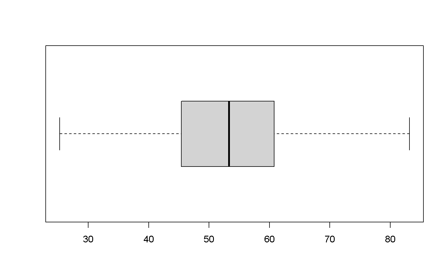
boxplot(x = nd, horizontal = T)
Key Points
Customize your graphs to make them more visually appealling.